Appearance
Daily Learning:RL
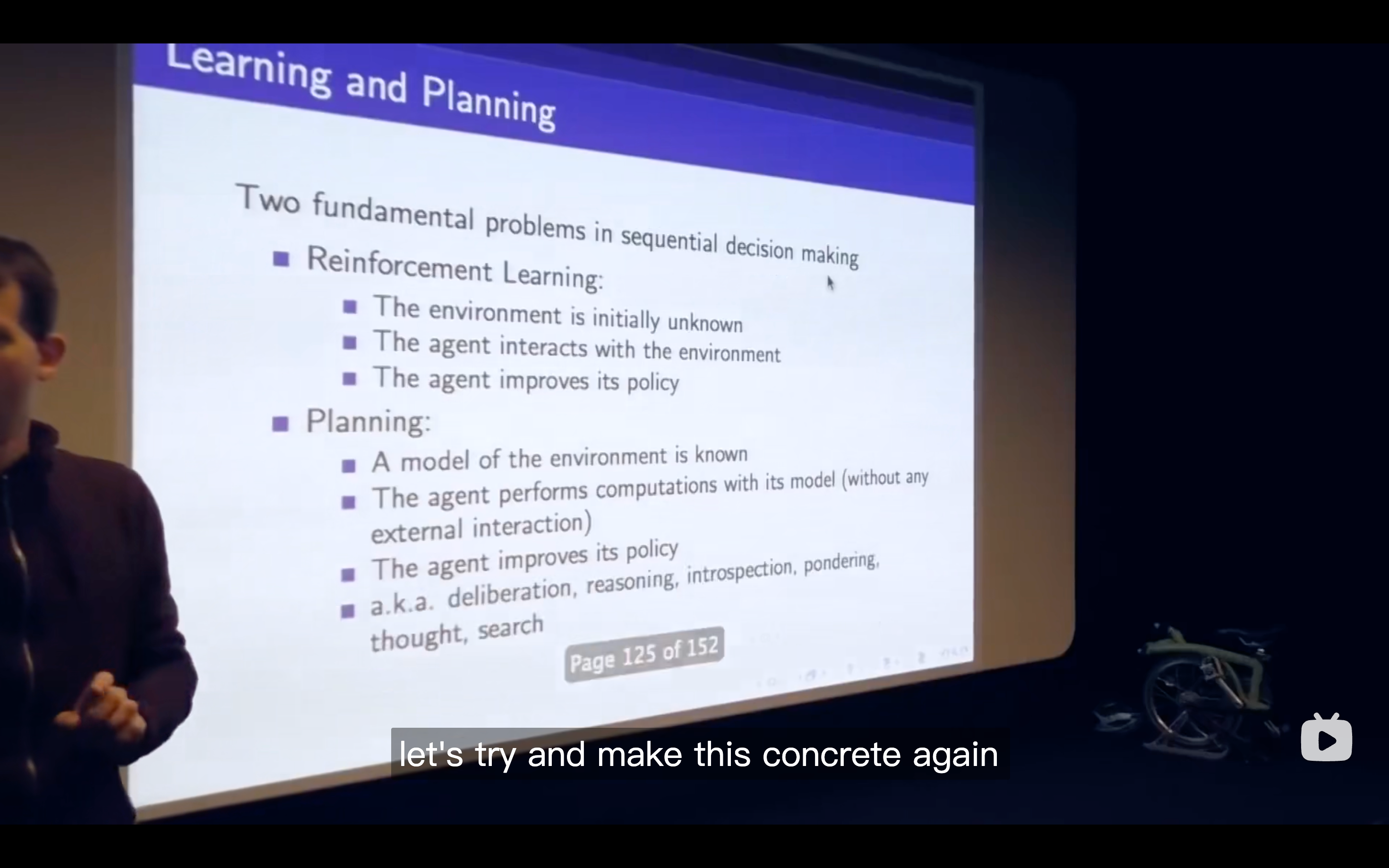
- Dynamic Programming 重点看
- Q learning 重点看
- Model free 重点看
- Value based 重点看 离散空间
- <u>policy based可以省略一点</u>
Lecture1: Intro to RL
[2025-11-04](file:///workspace/d047dbd0-d7d7-404e-8dc2-62572c04acd5/wl-Rrmz1Mj5CWeLLEwT_3)
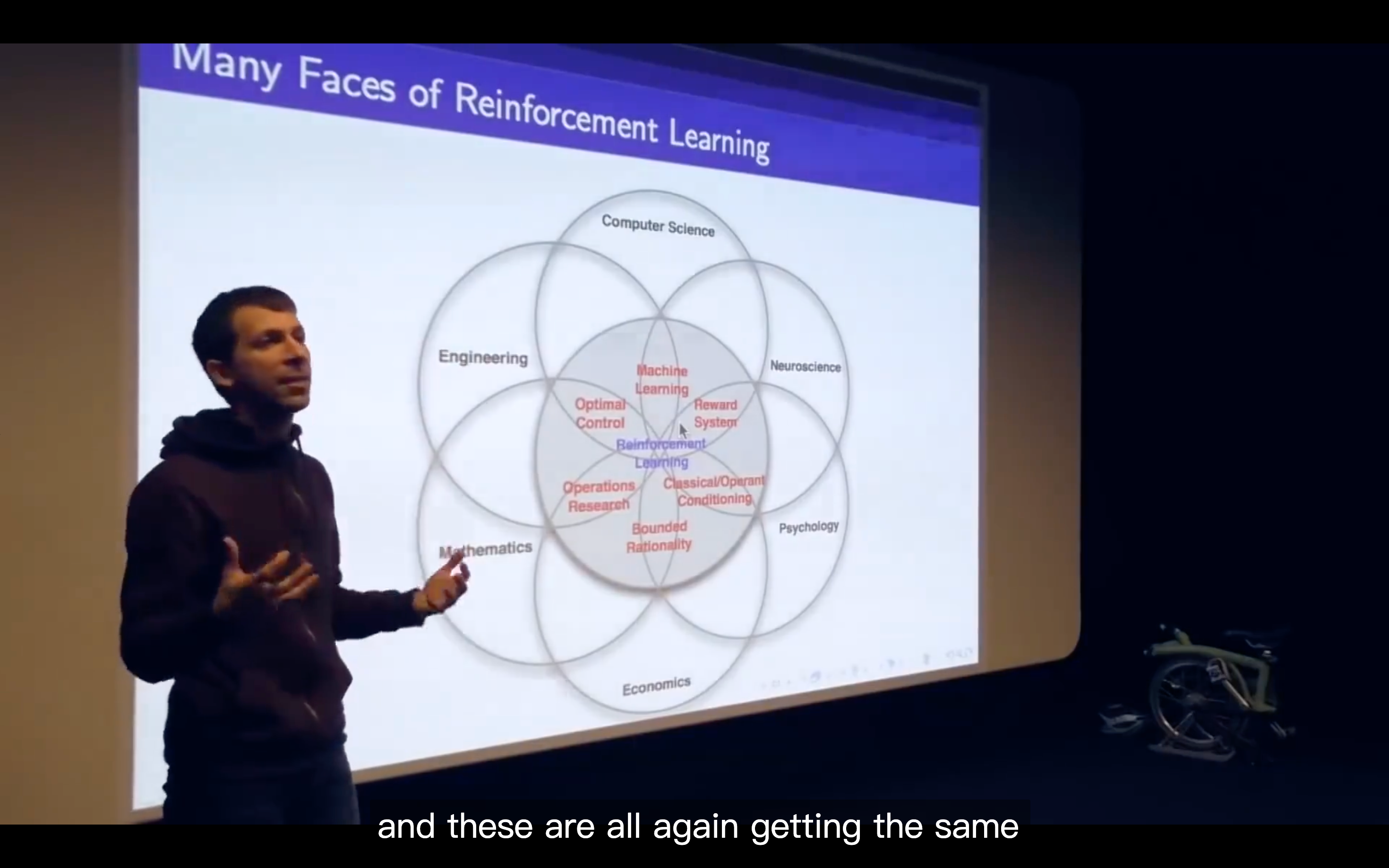
- Characteristics of RL
- There's no supervisor, but only a reward signal
- Feedback is delayed, not instantaneous
- Time really matters
- Agent's actions affect the subsequent data it receives
- What we need is to figure out the algorithm in the Agent's "mind"
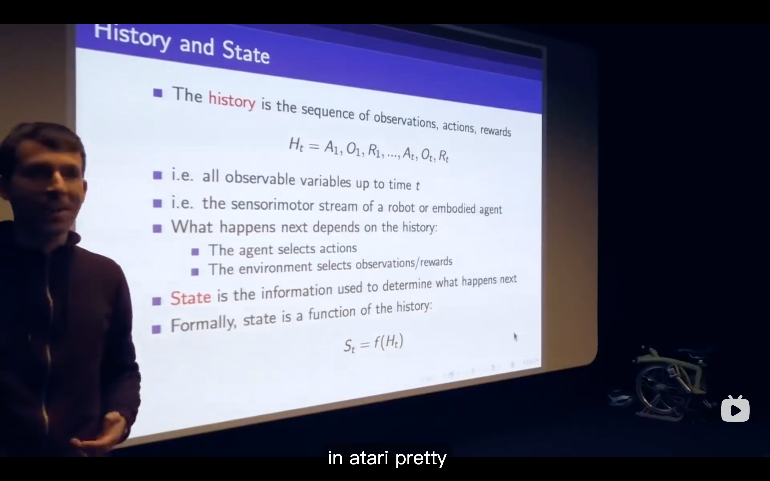
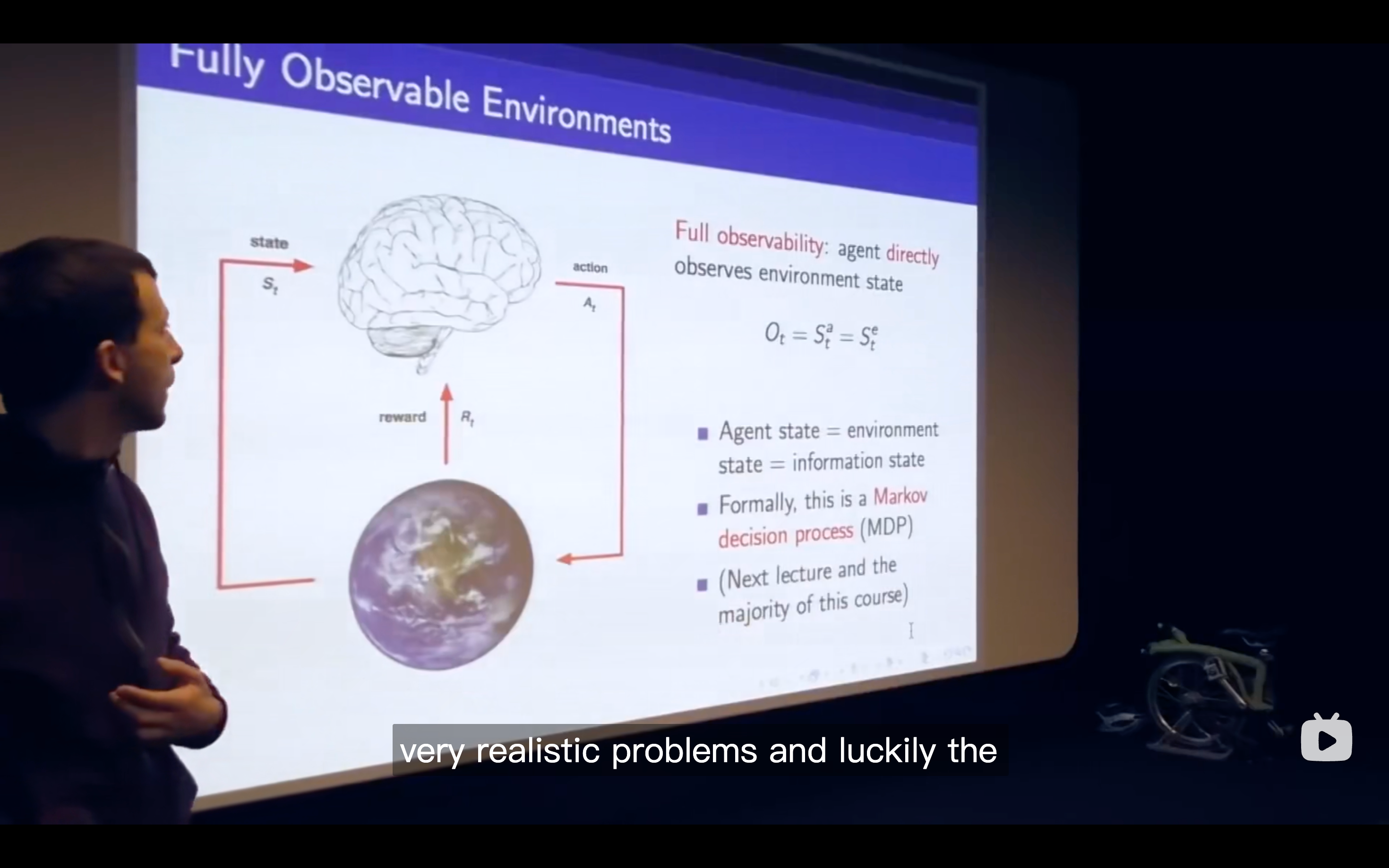
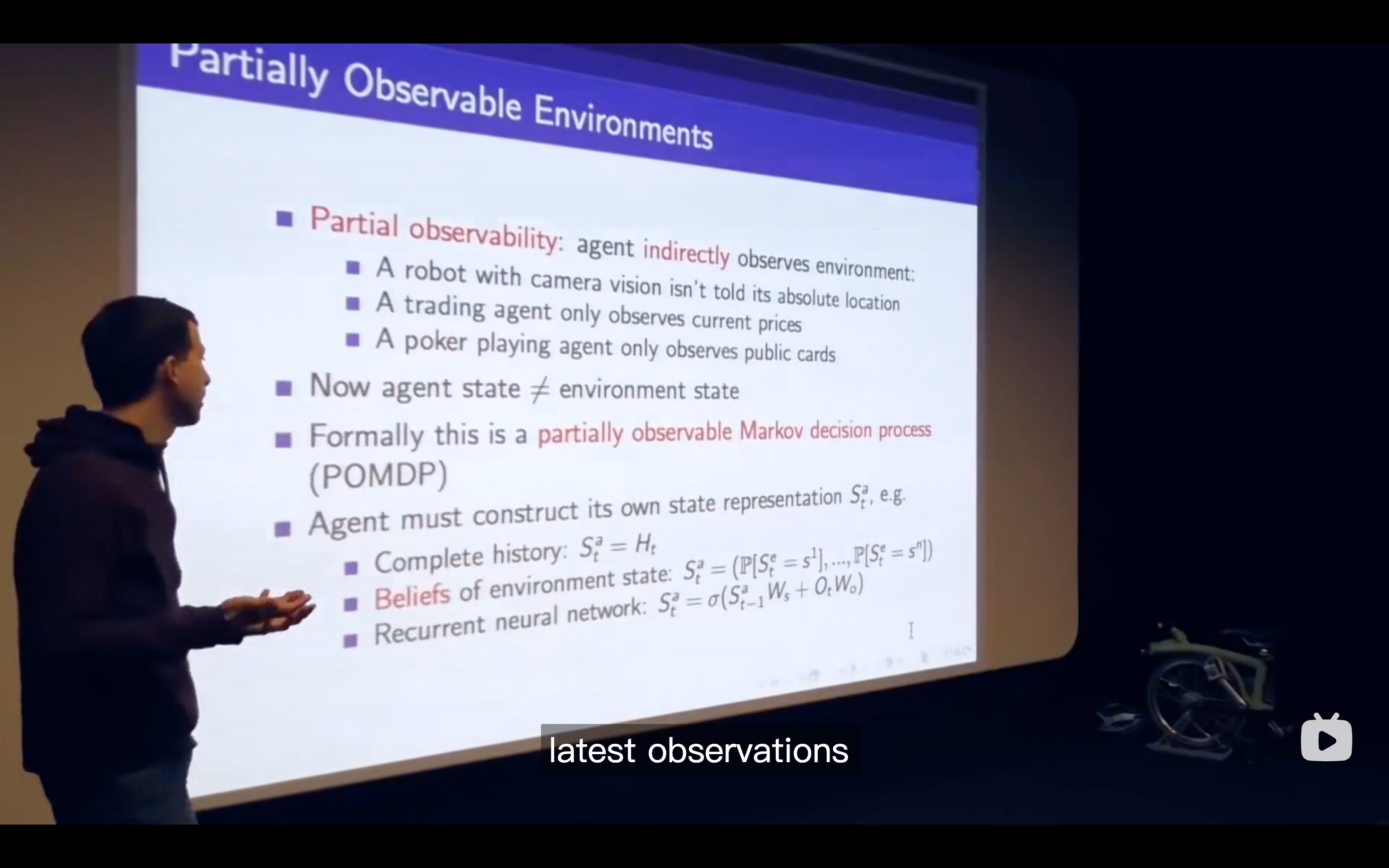
- The valid definition of state would be to only look at the last observation
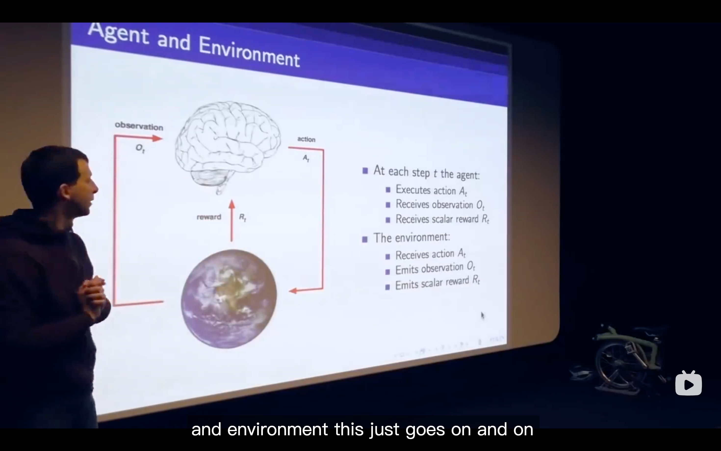
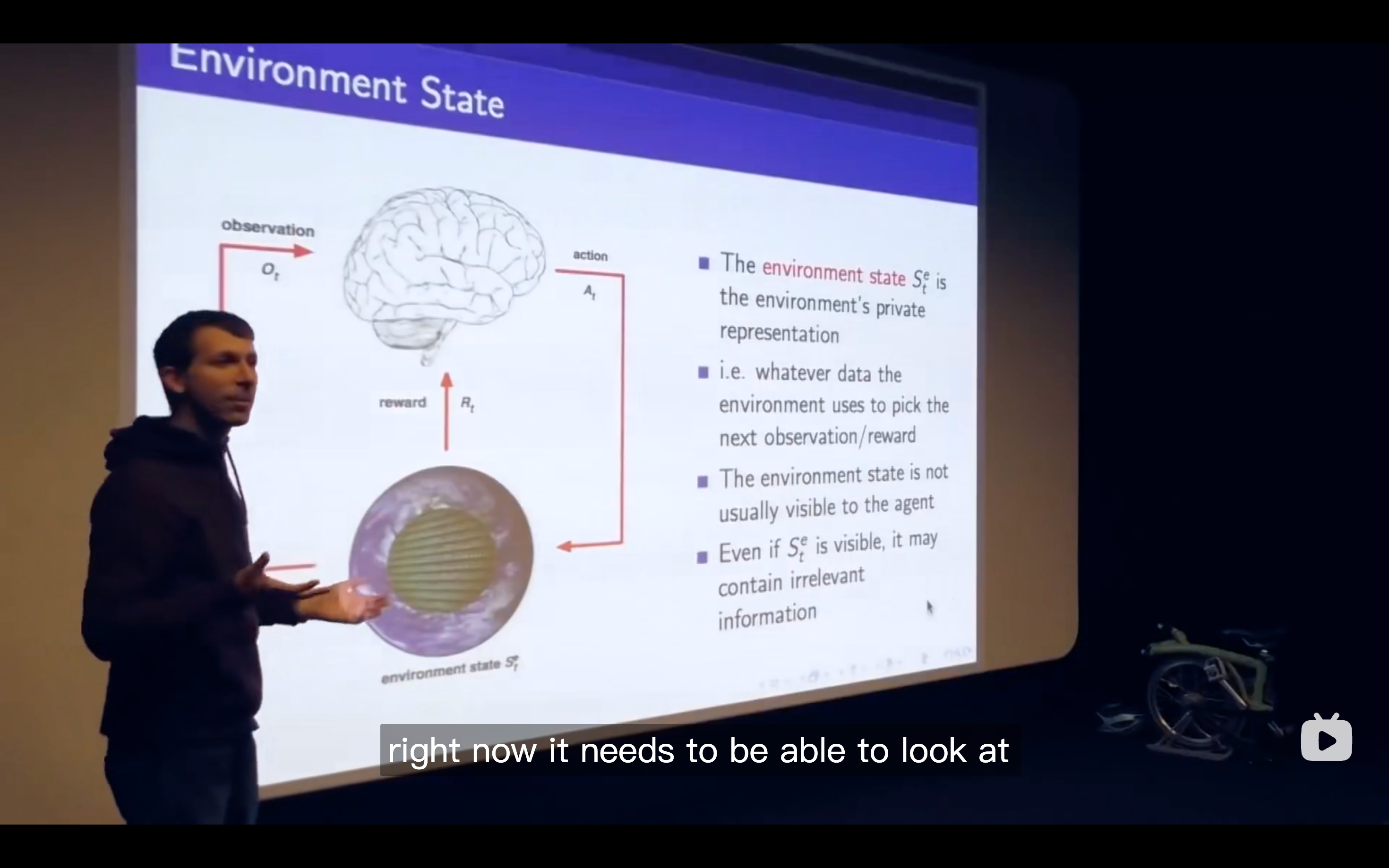
Environment State
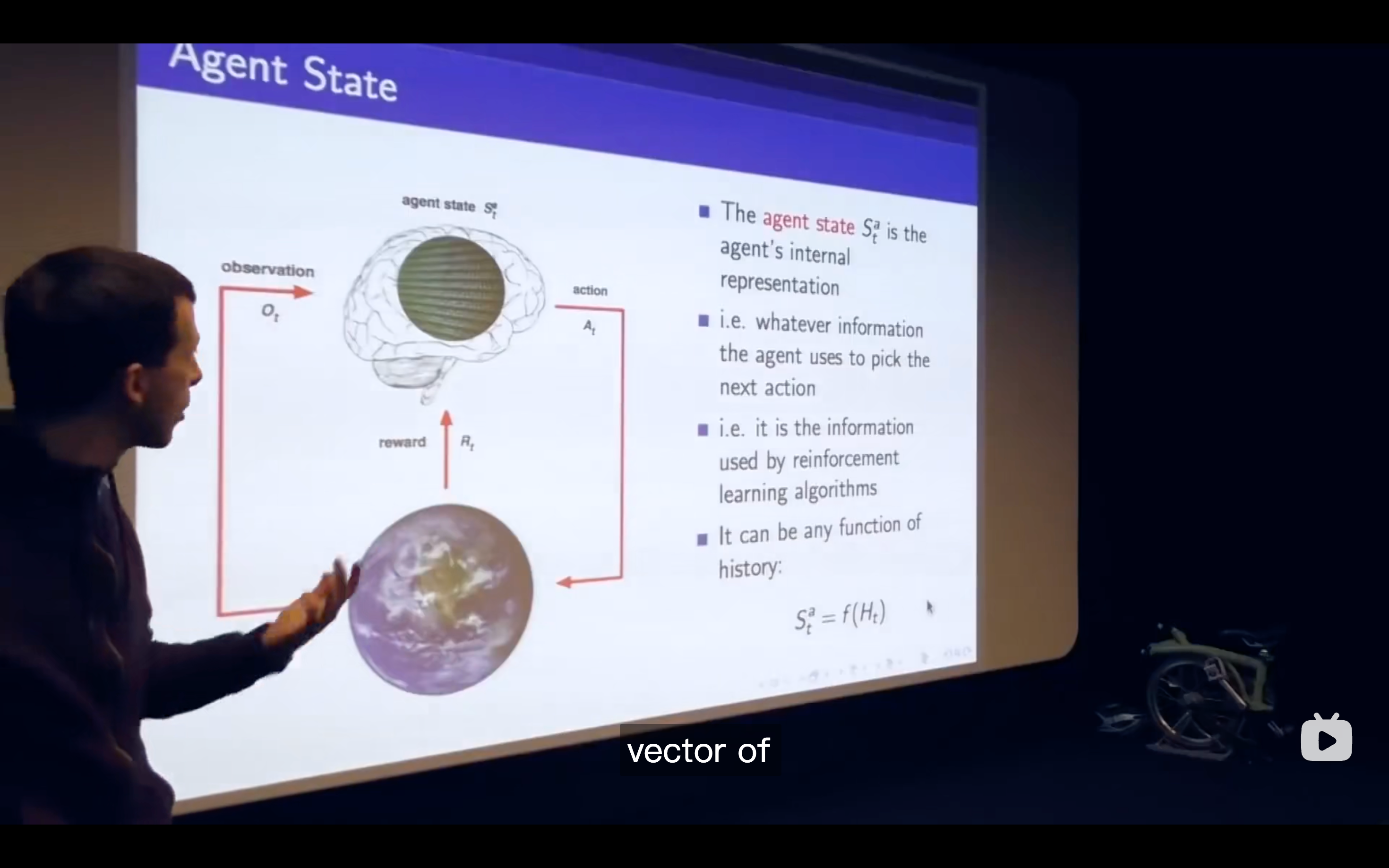
Agent State
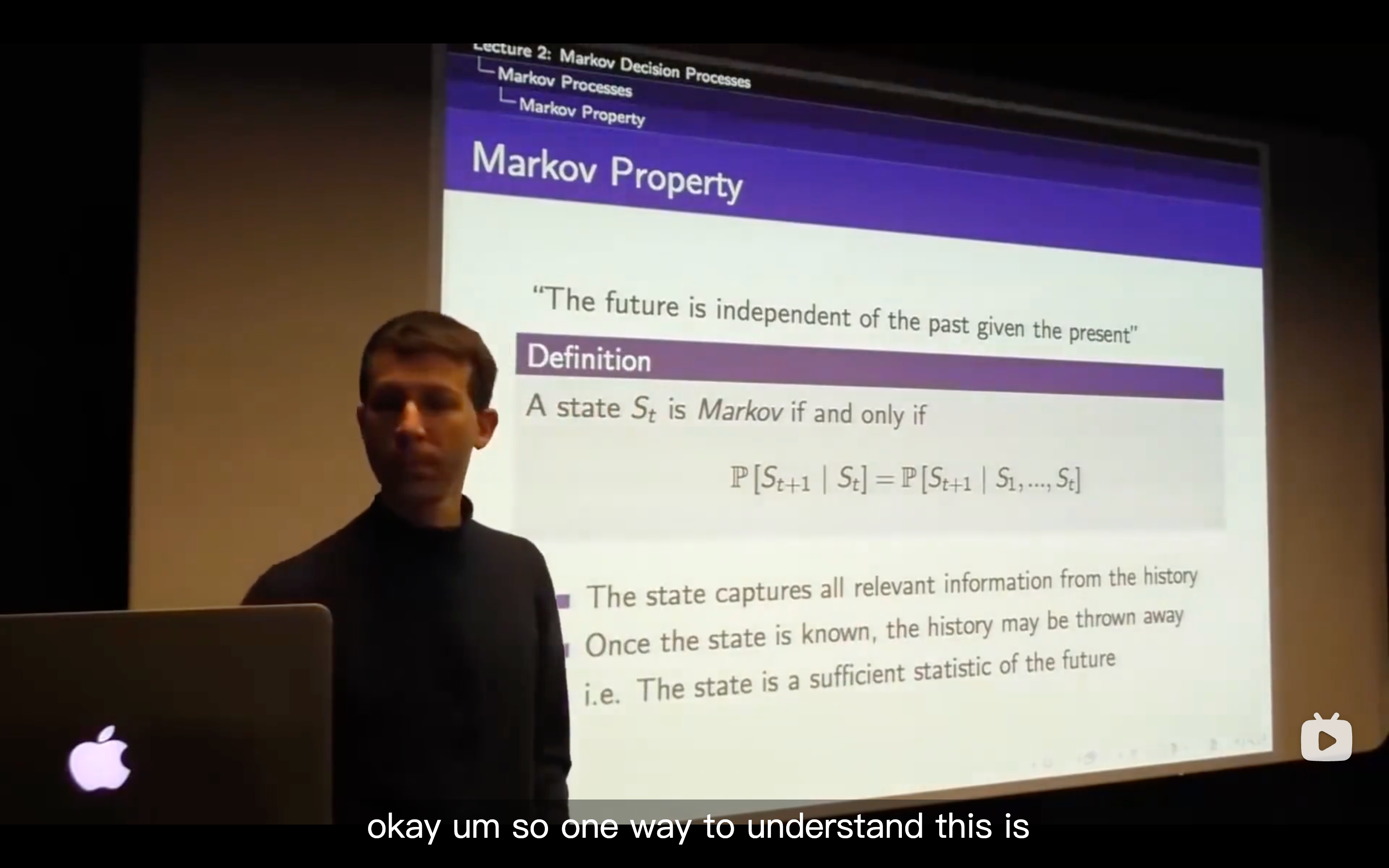
Information(Markov) State
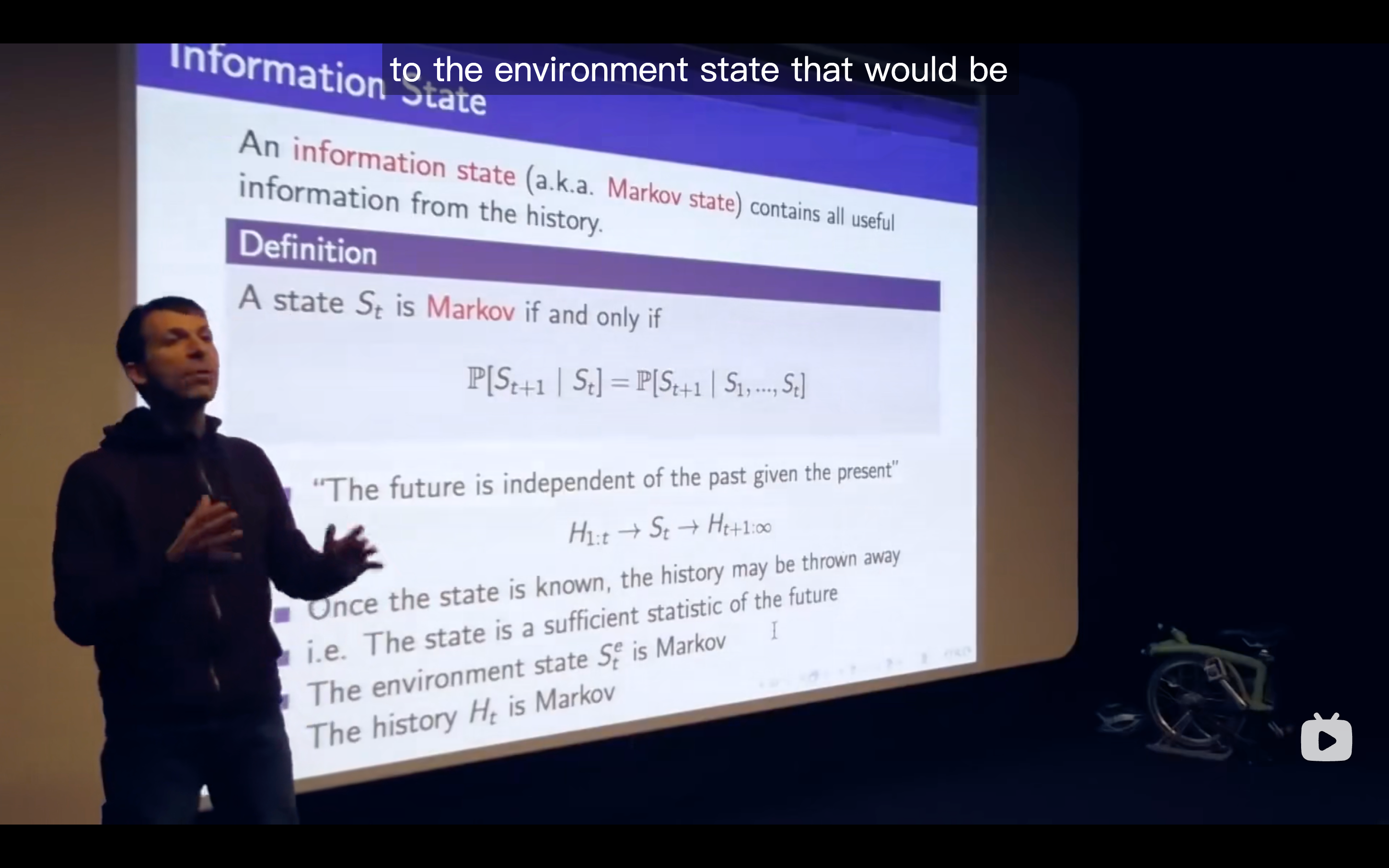
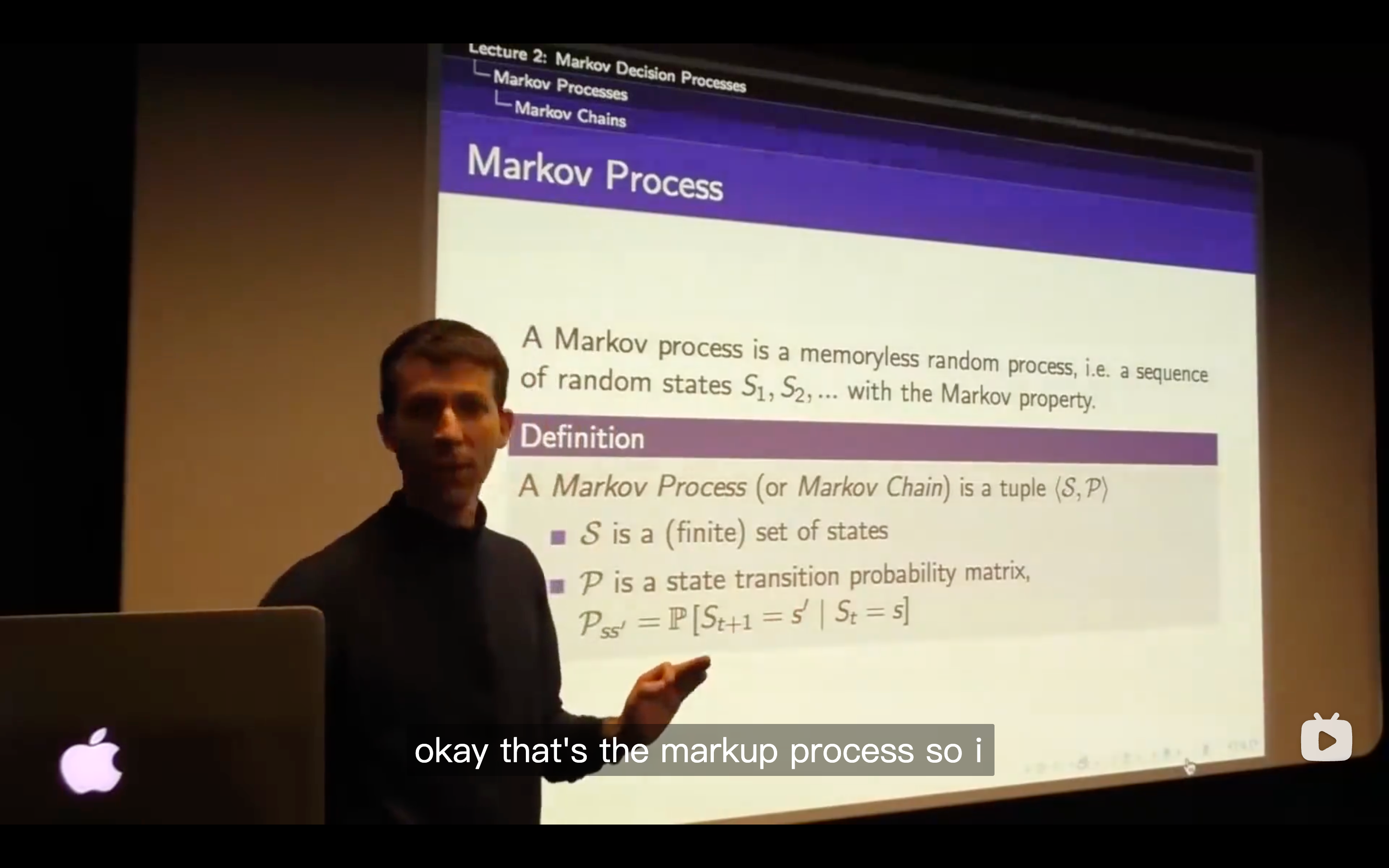
- The Markov state contains enough information to characterize all future rewards
- The Markov state contains enough information to characterize all future rewards
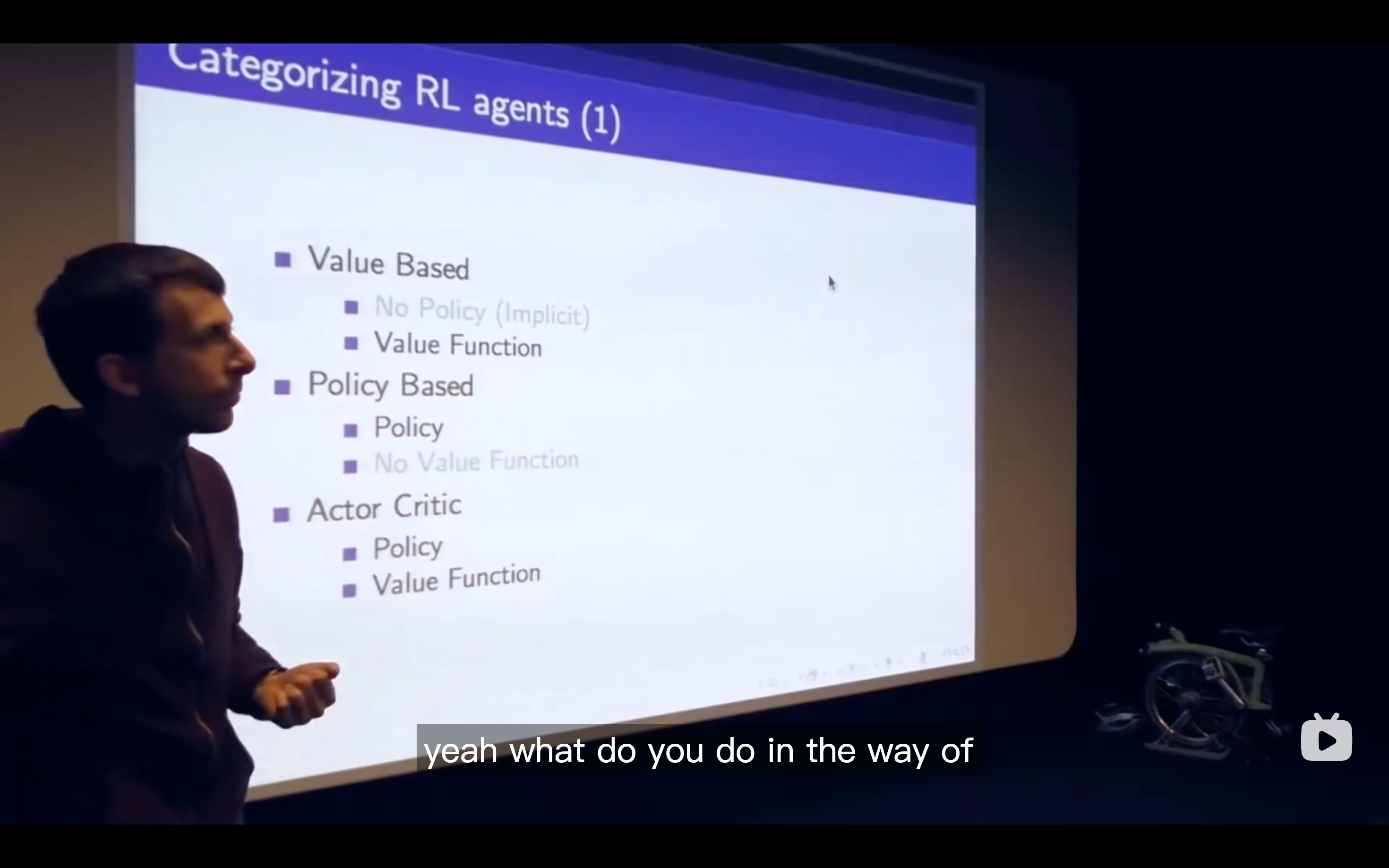
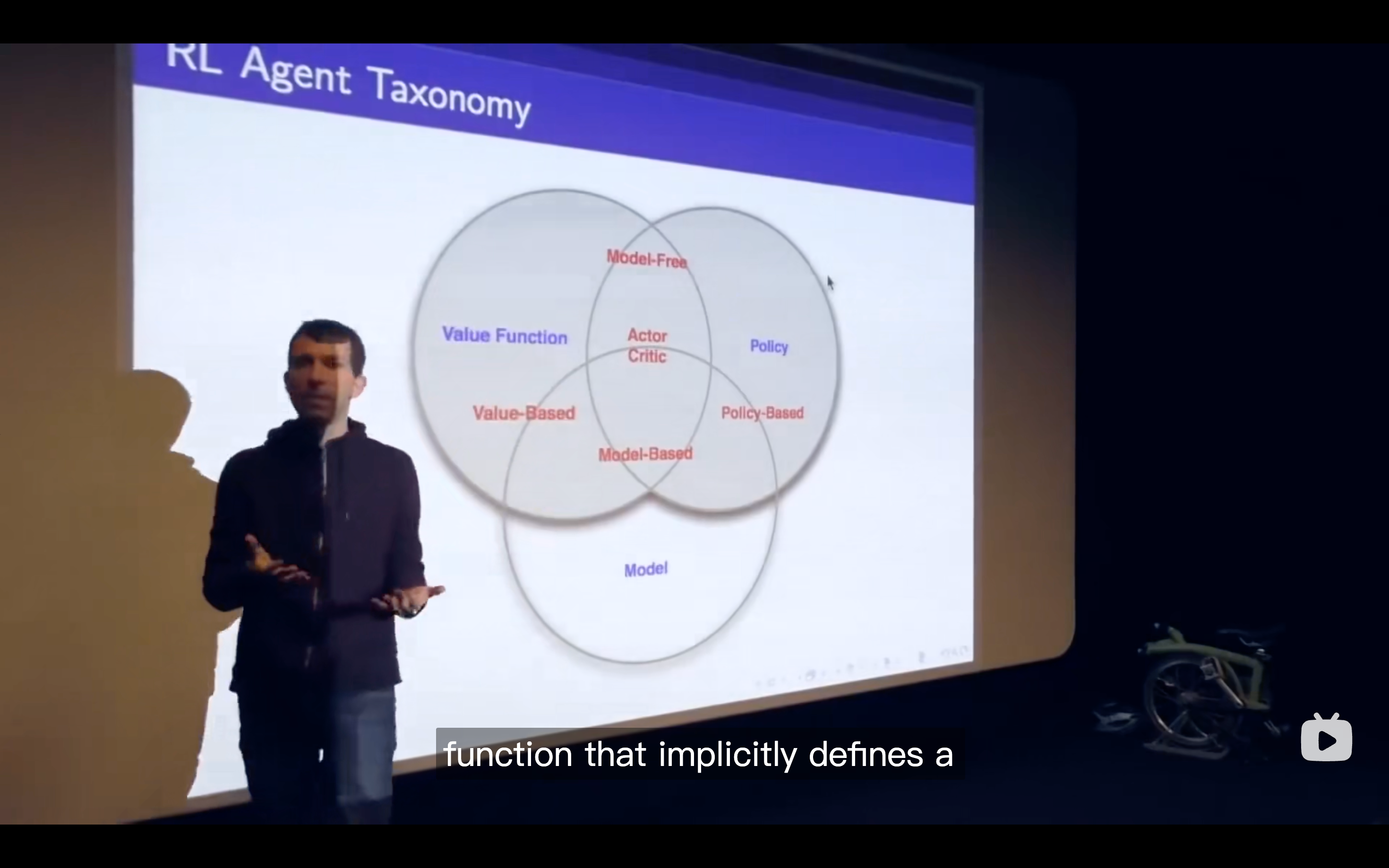
Major Components of an RL Agent
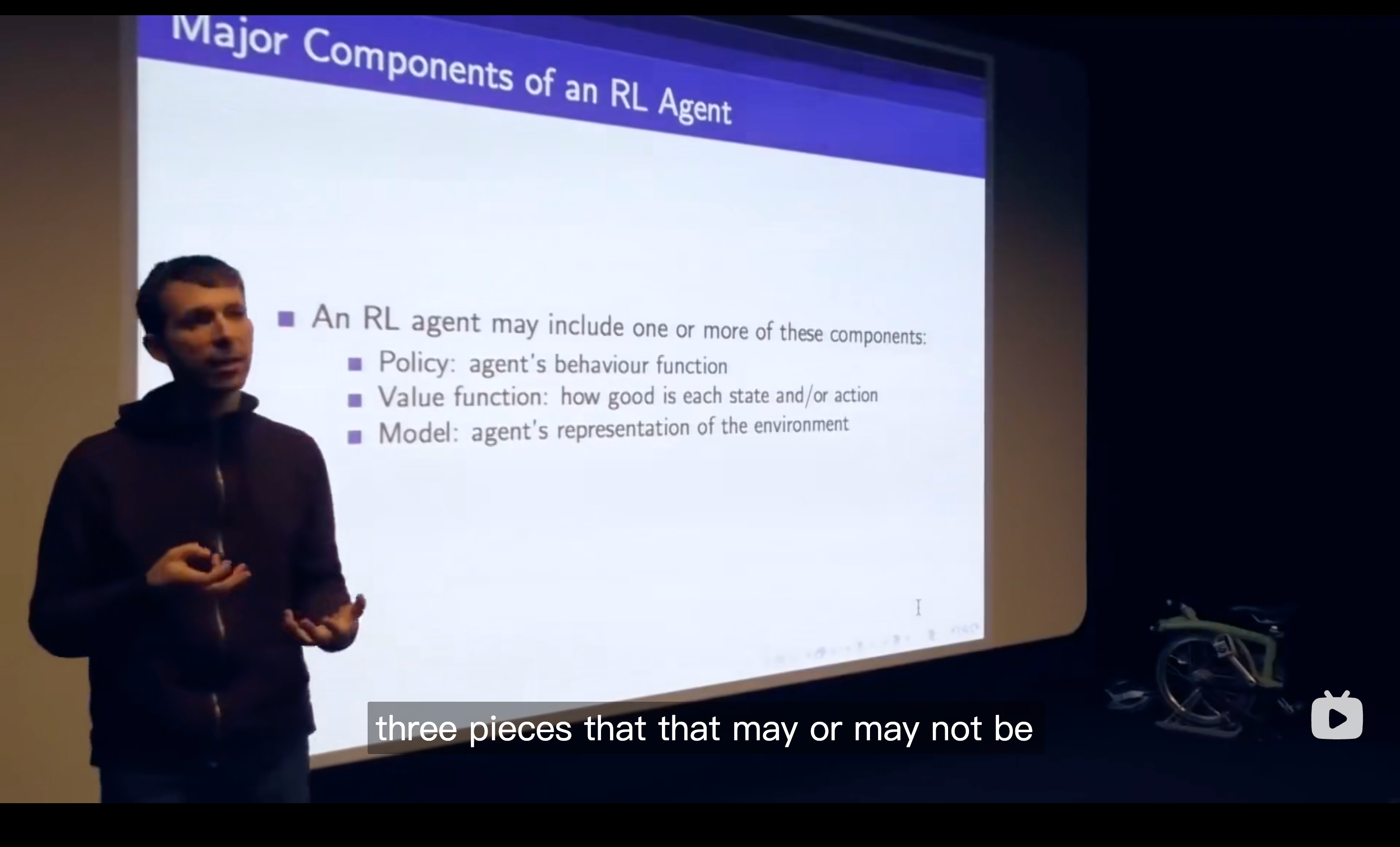
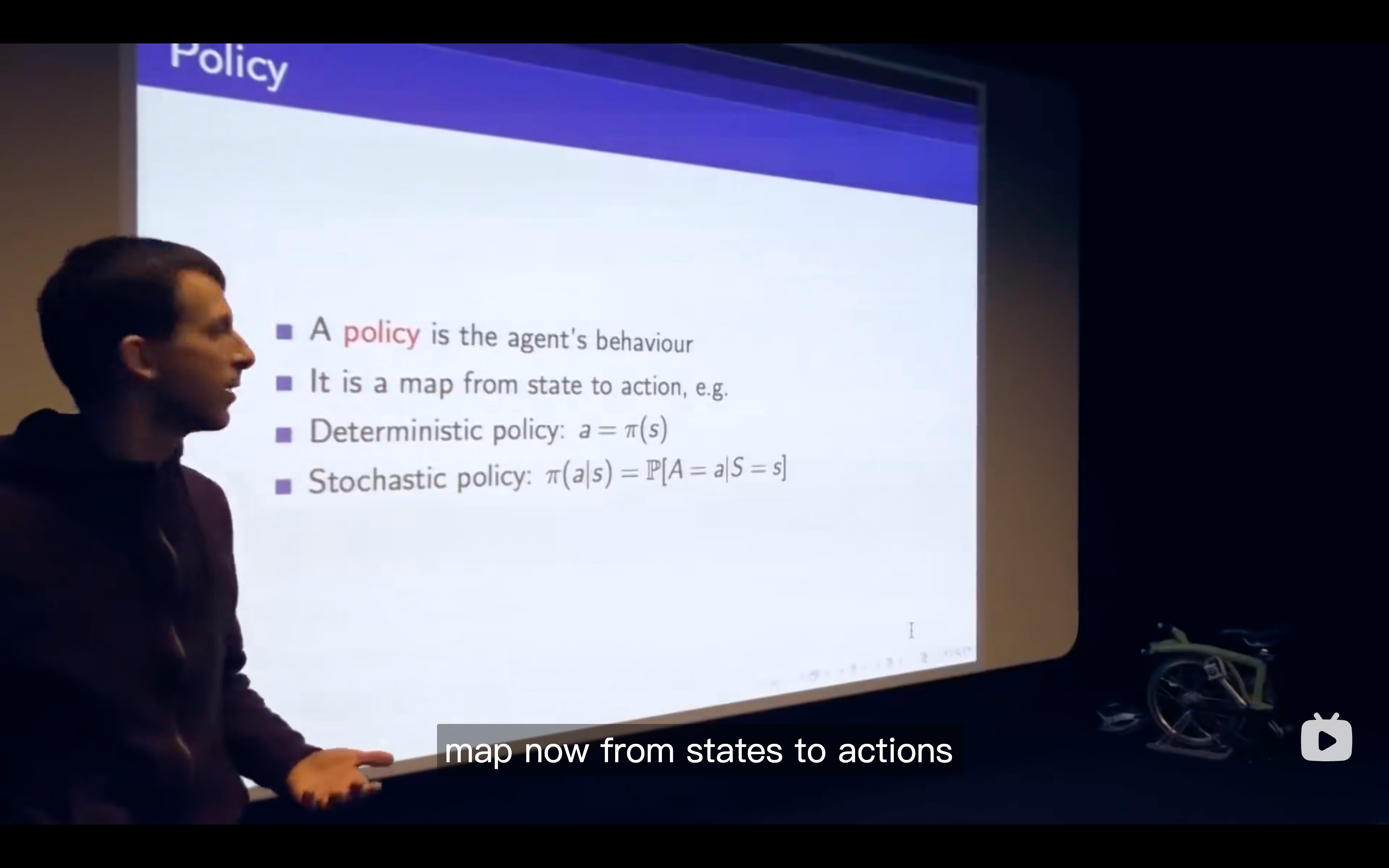
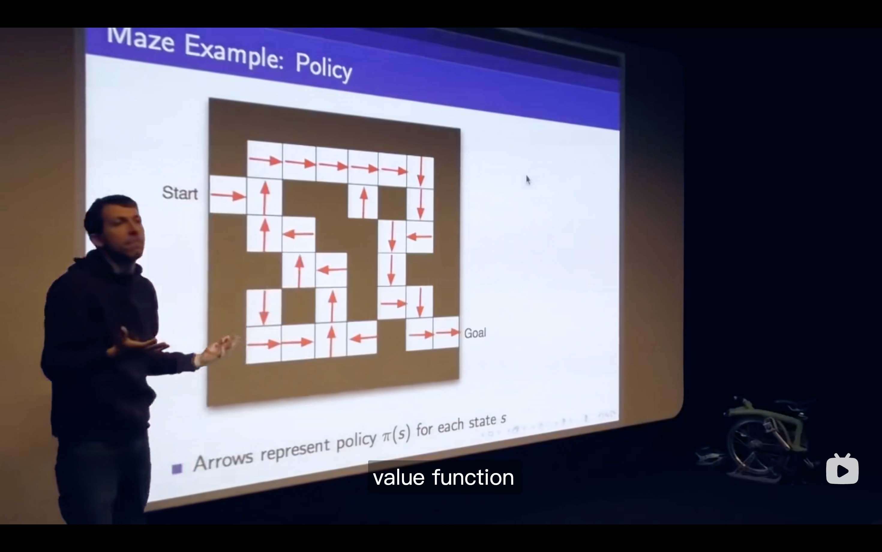
Policy
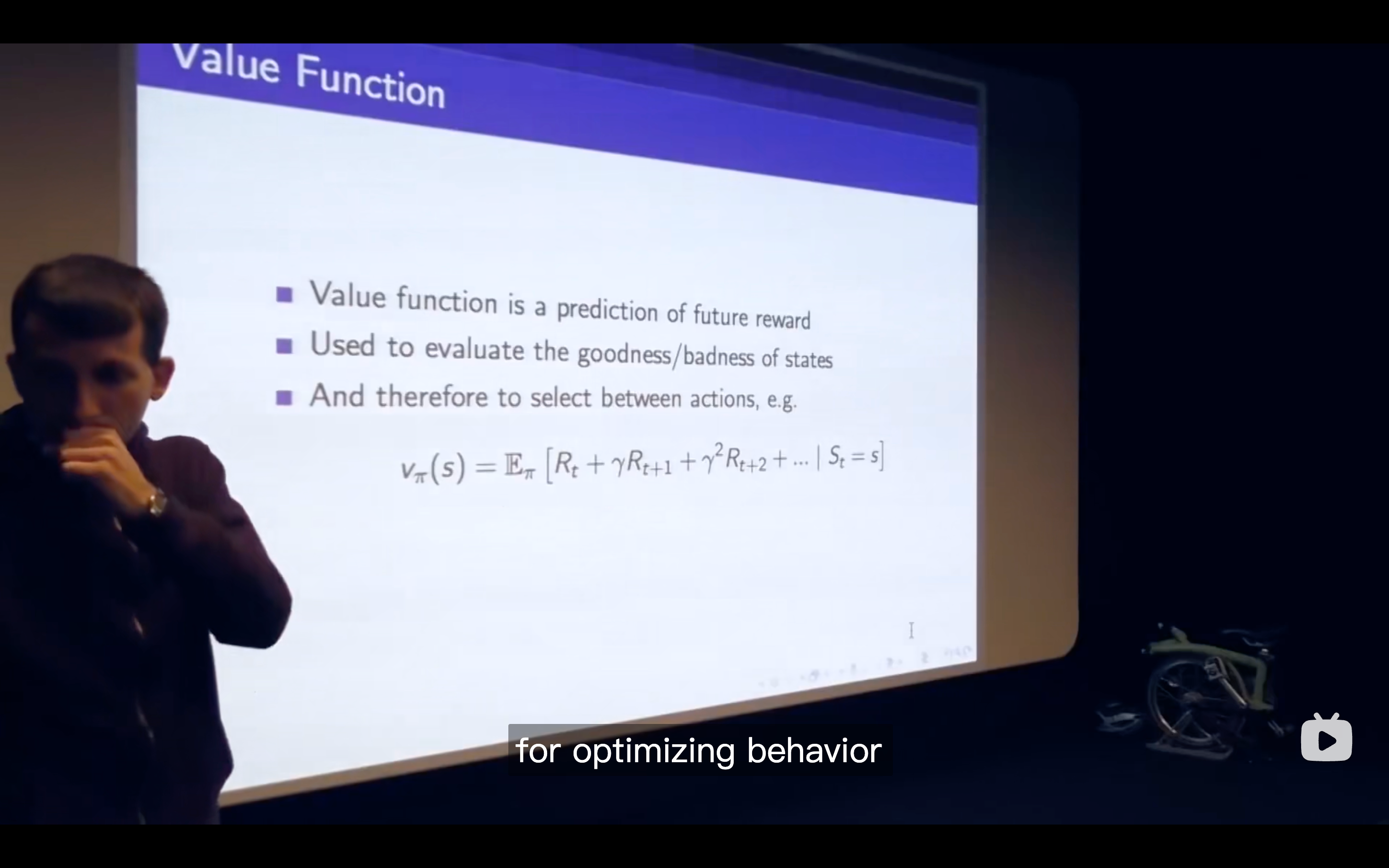
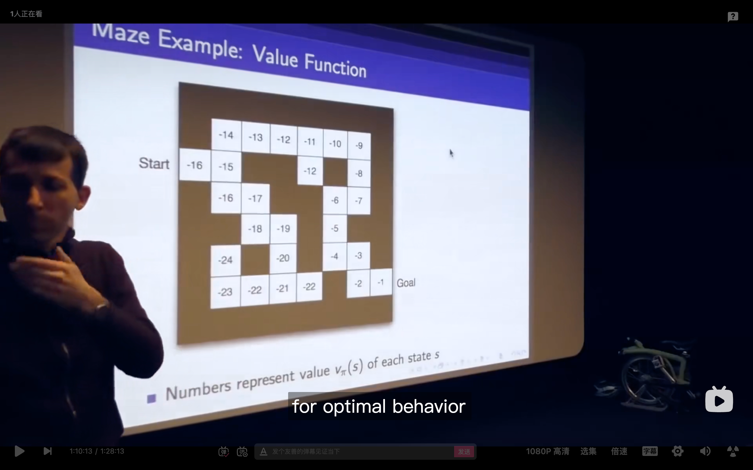
Value function
- The behavior that maximizes the value is the one that correctly trades off the agent's risks so as to get the maximum amount of reward going into the future, and that just automatically emerges from the performance.
- The behavior that maximizes the value is the one that correctly trades off the agent's risks so as to get the maximum amount of reward going into the future, and that just automatically emerges from the performance.
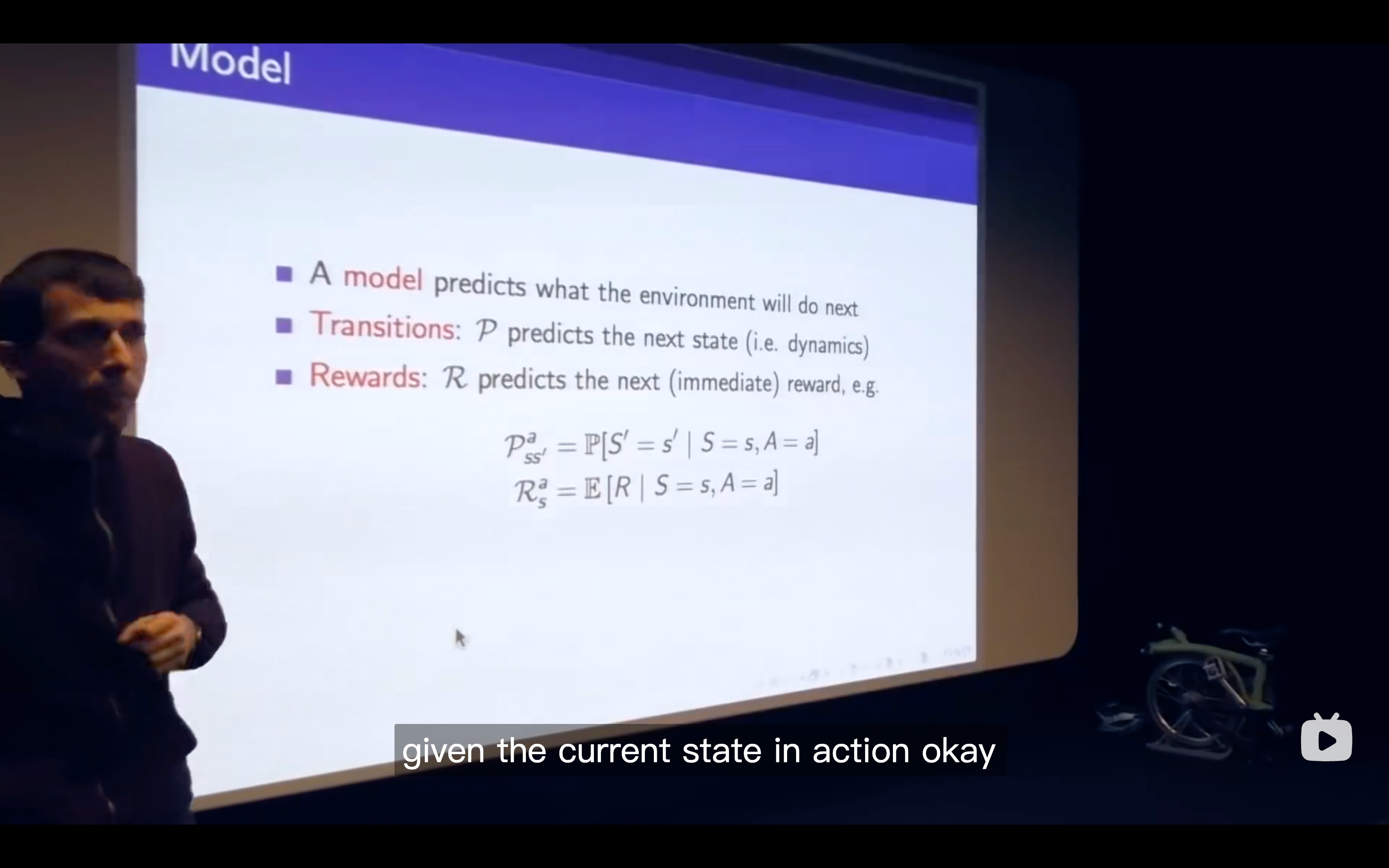
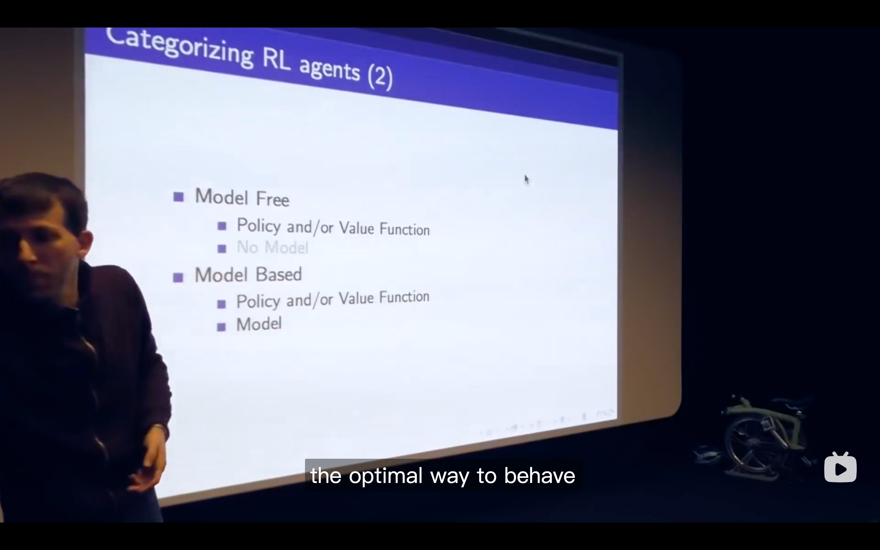
Model
- RL is like trial-and-error learning
- The agent should discover a good policy
- From its experiences of the environment
- Without losing too much reward along the way
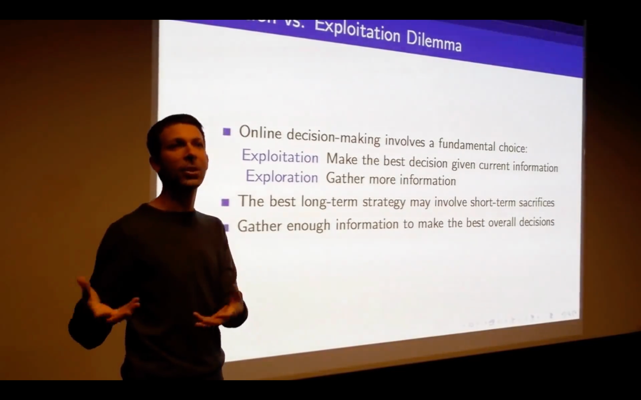
- Exploration & Exploitation
- Exploration finds more information about the environment
- choosing to give up some reward that you know about in order to find more about the environment
- Exploitation exploits known information to maxmise reward
- It's usually important to explore as well as exploit
- Exploration finds more information about the environment
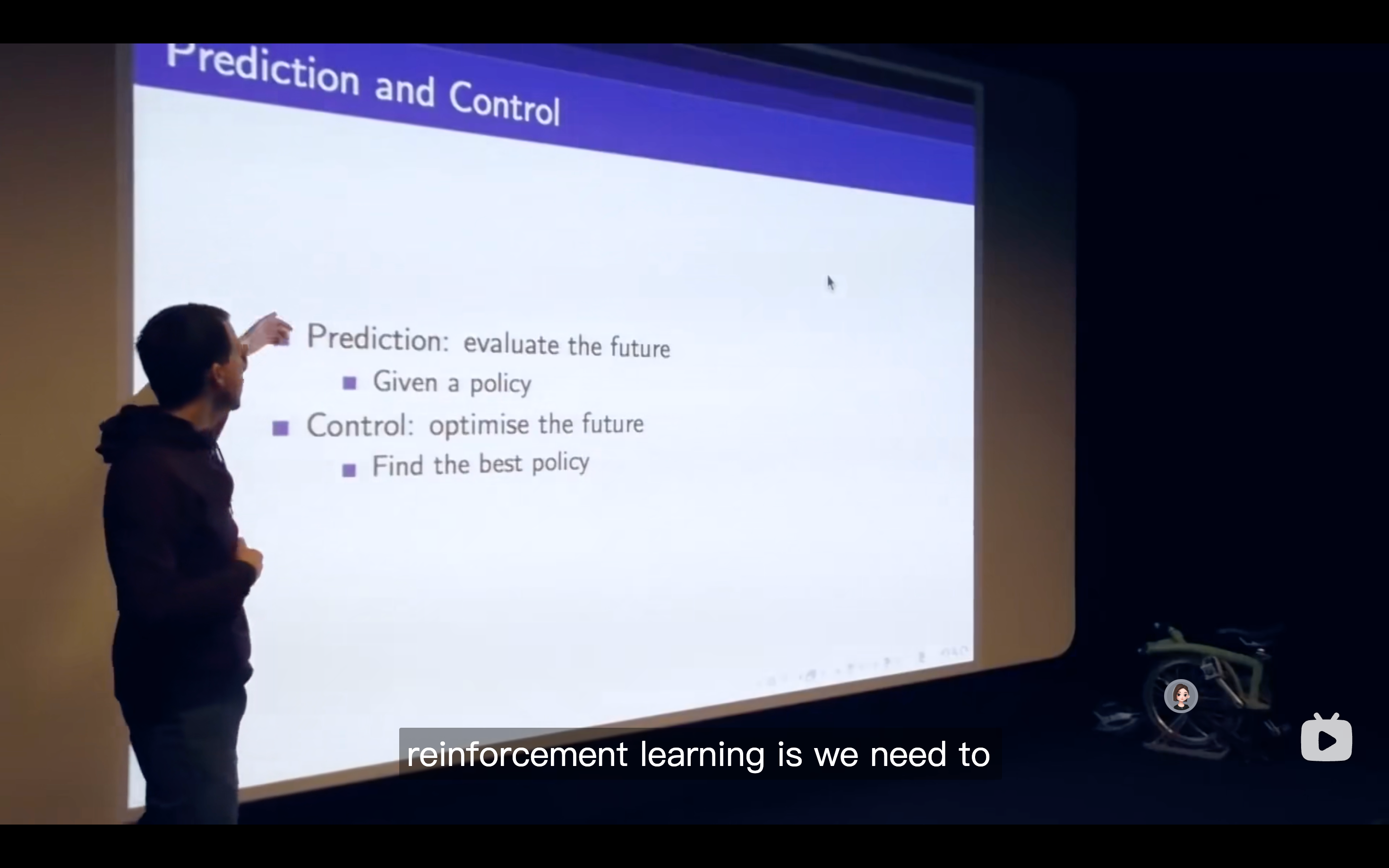
- RL is we need to solve the prediction problem in order to solve the control problem which means we need to evaluate all of the policies to find the best one.
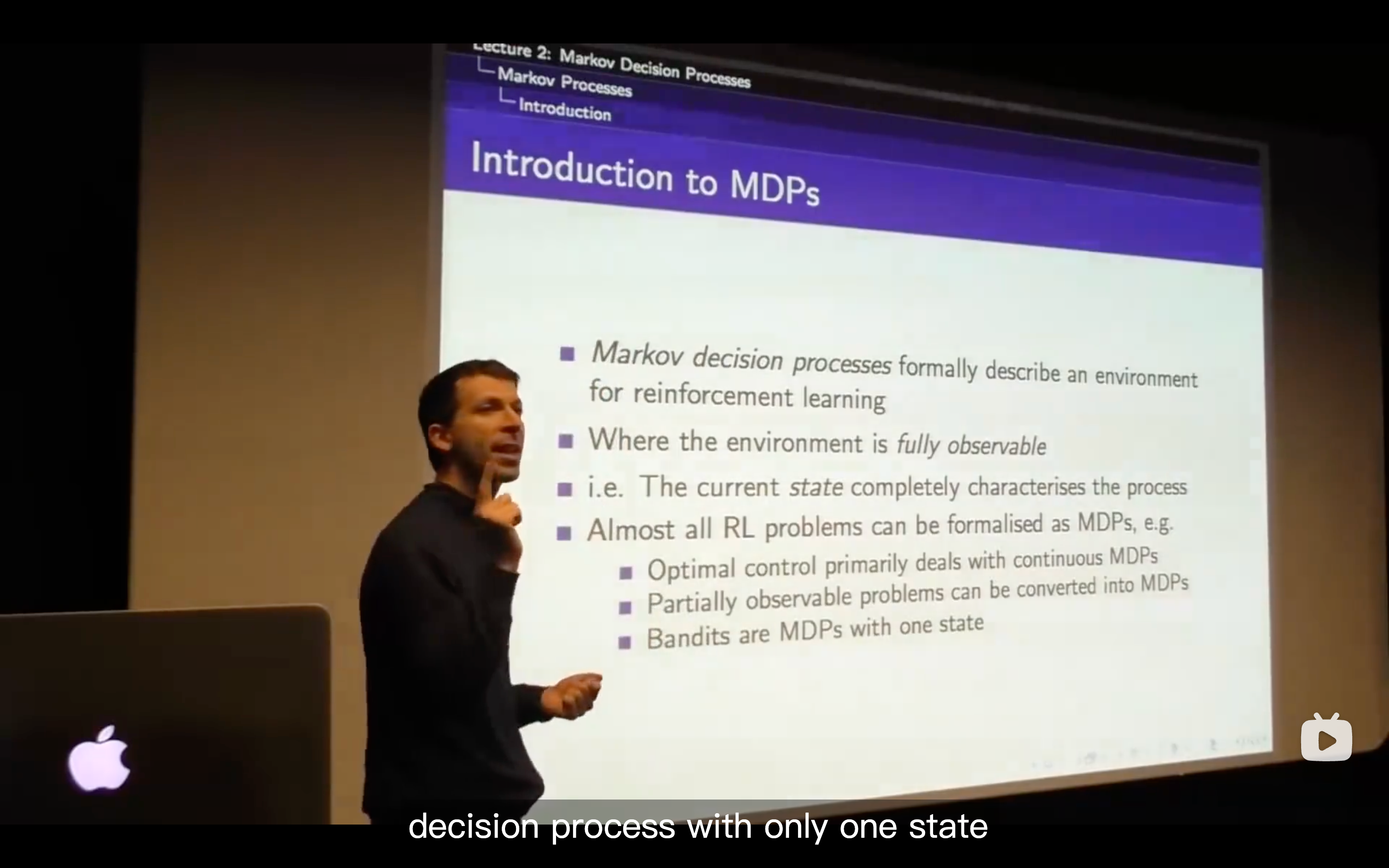
Lecture2: Markov Decision Process
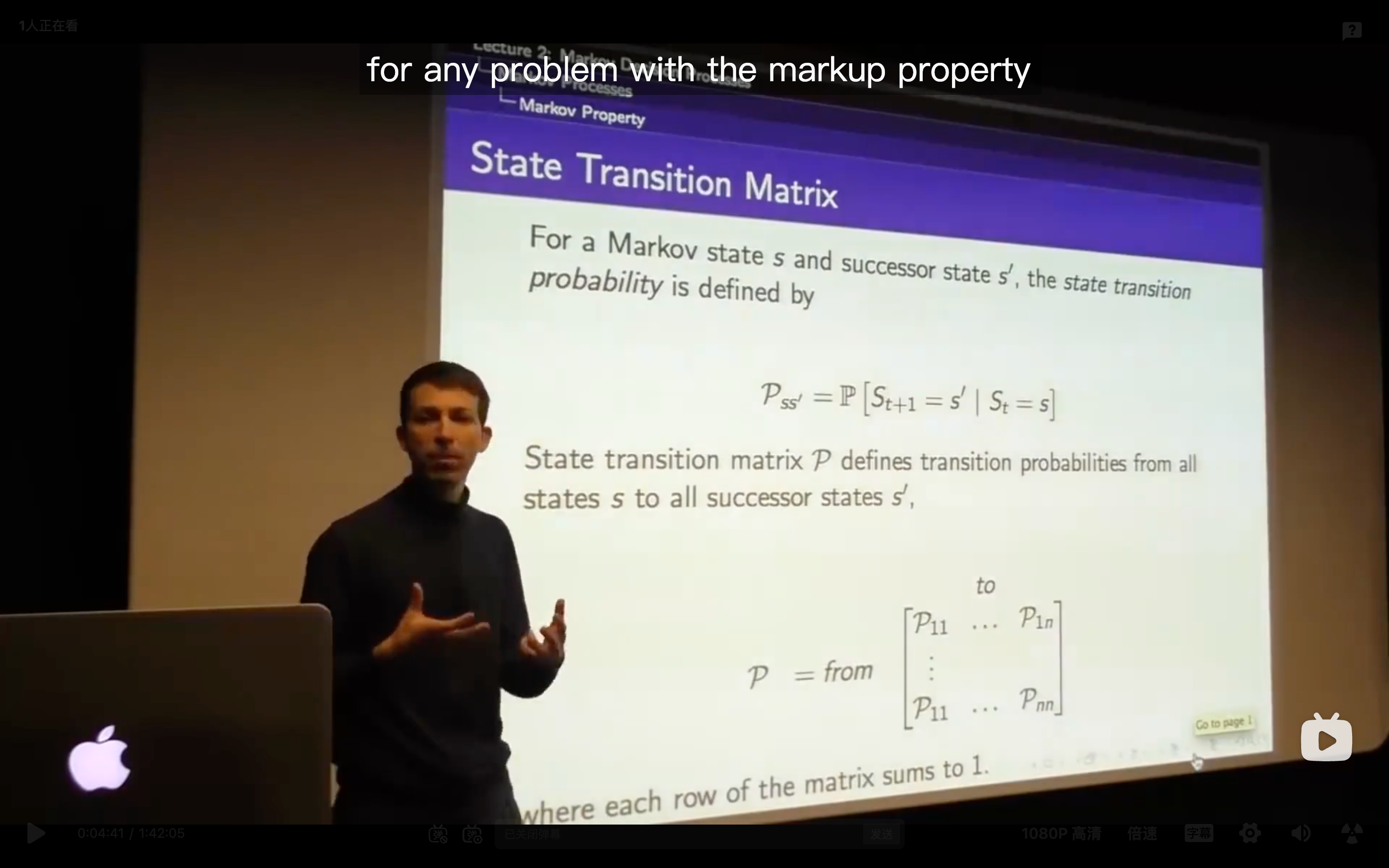
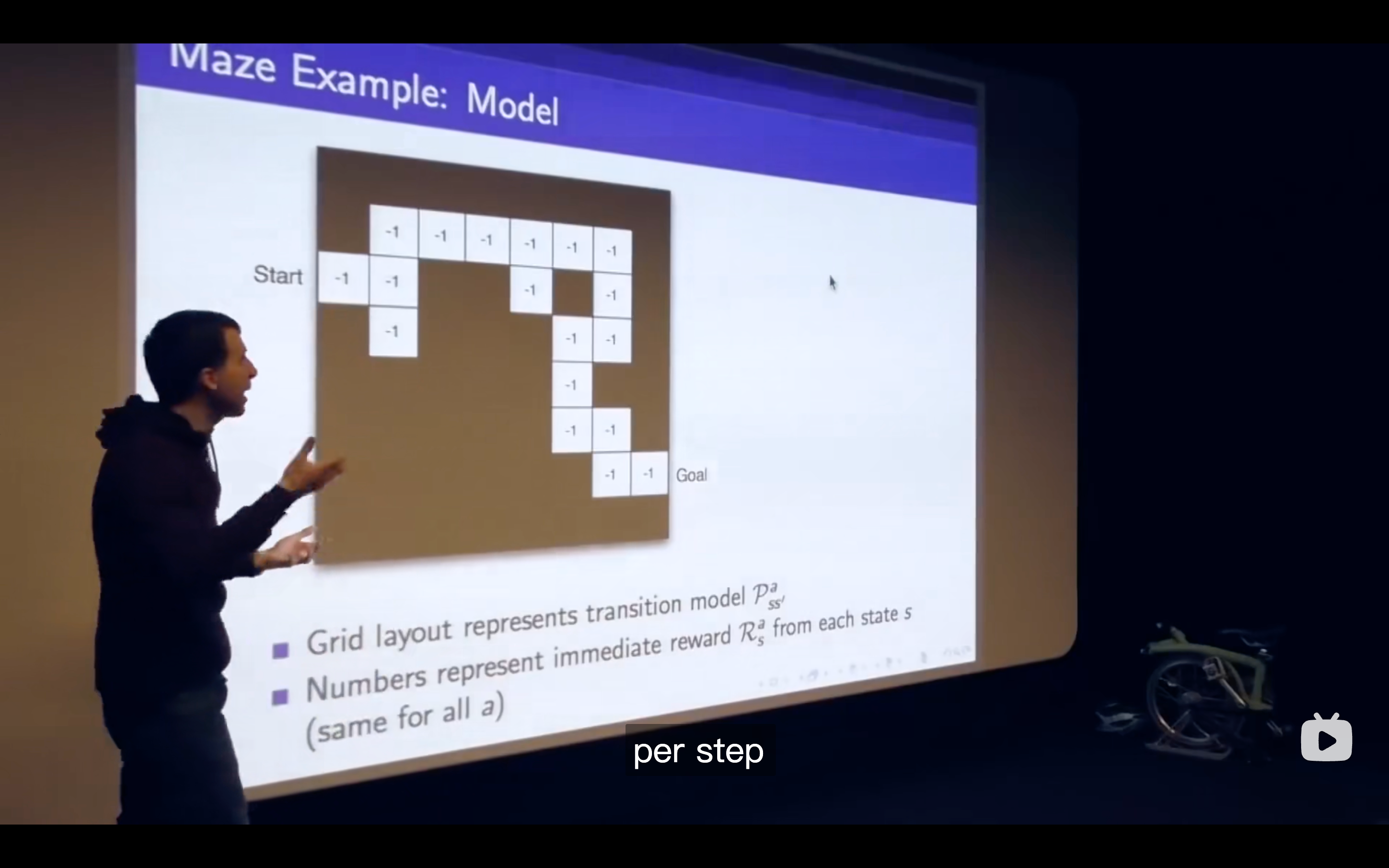
- Each row of this matrix tells us what will happen for each state that I was in.
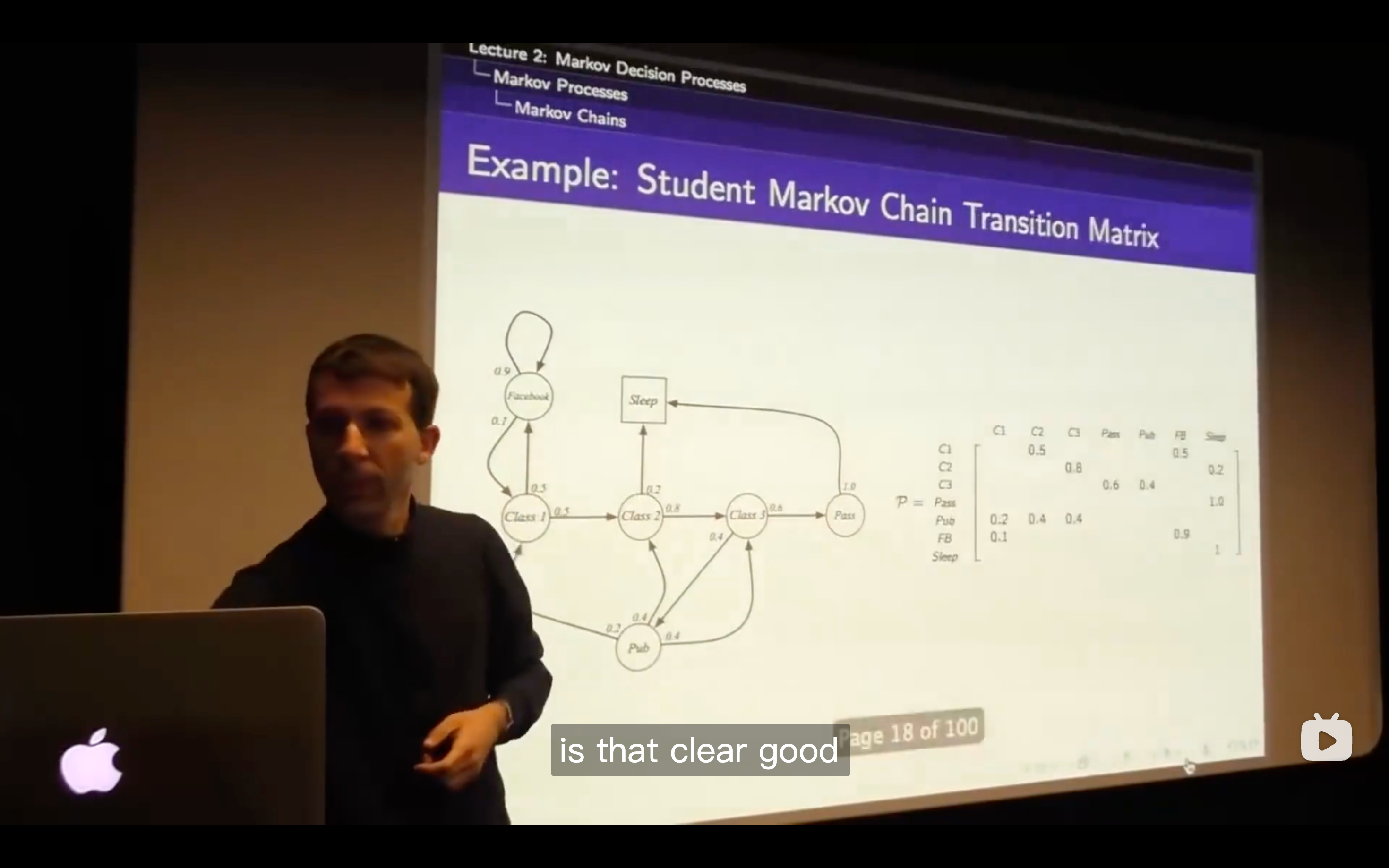
This example gives an explicit explanation for how the matrix was built
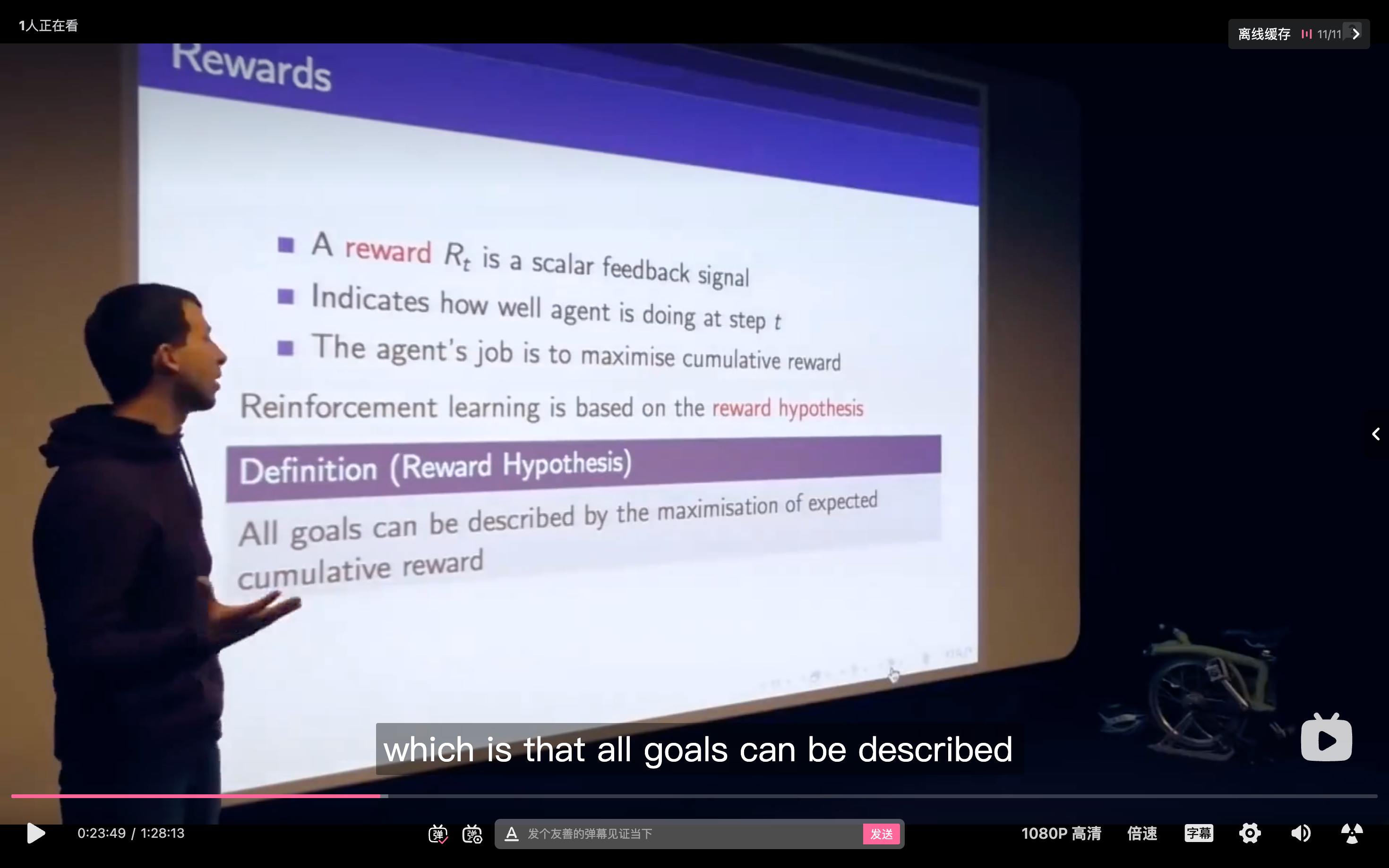
Markov Reward Process.
- It is the Markov process with some value judgement
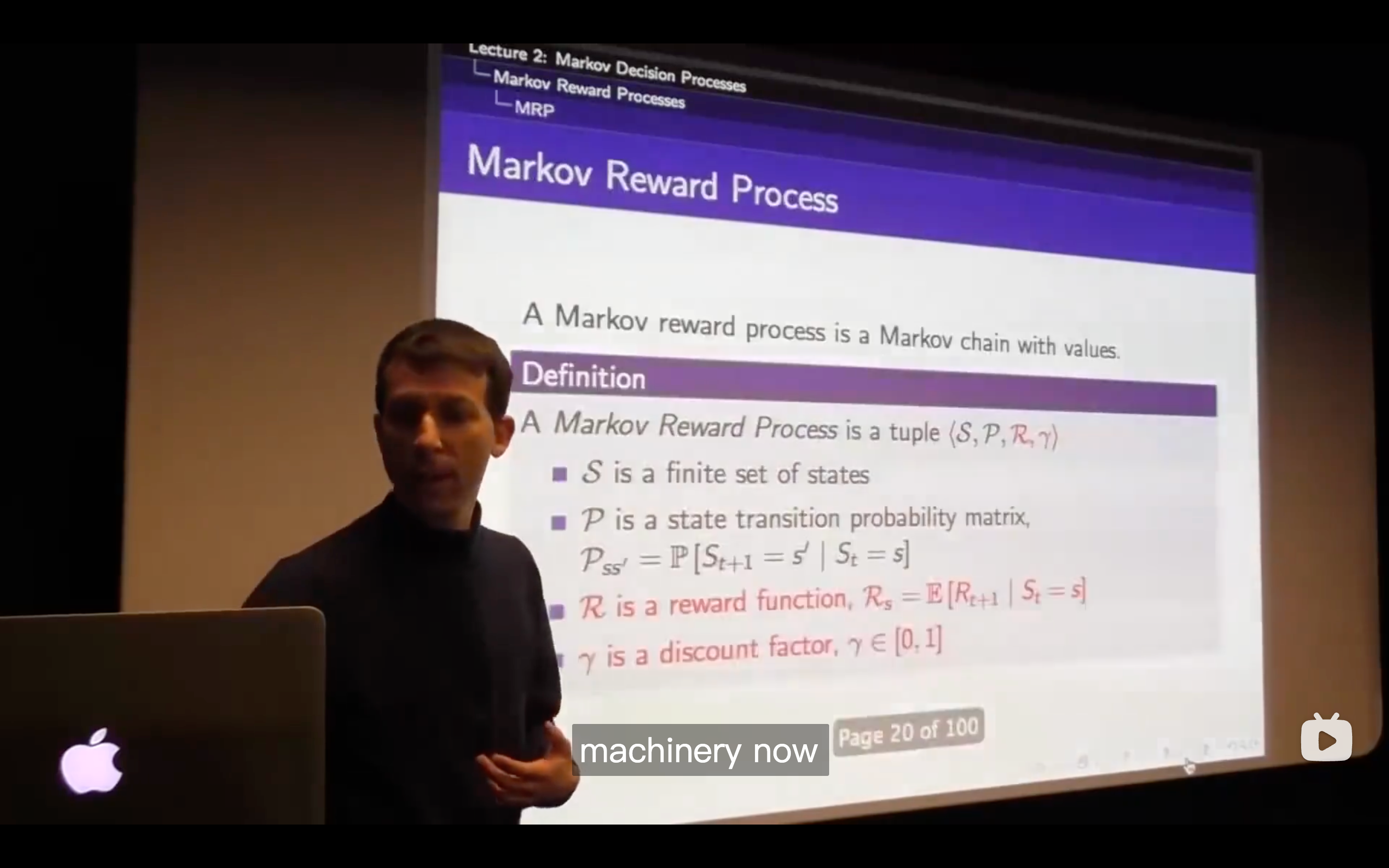
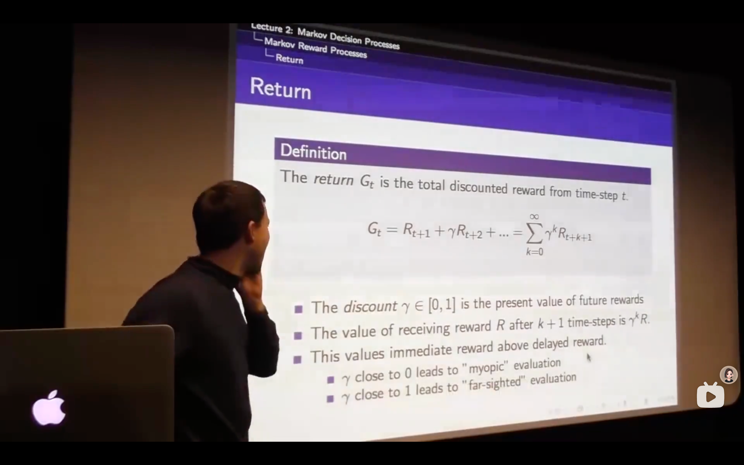
refers to the"goal", the goal is to maximize the sum of all of these rewards - For
: - 0 kind of means maximally short-sighted, which shows that you basically zero anything beyond your current time step and you only look at that first reward
- 1 is maximally fast sighted where you care about all rewards going infinitely far into the future
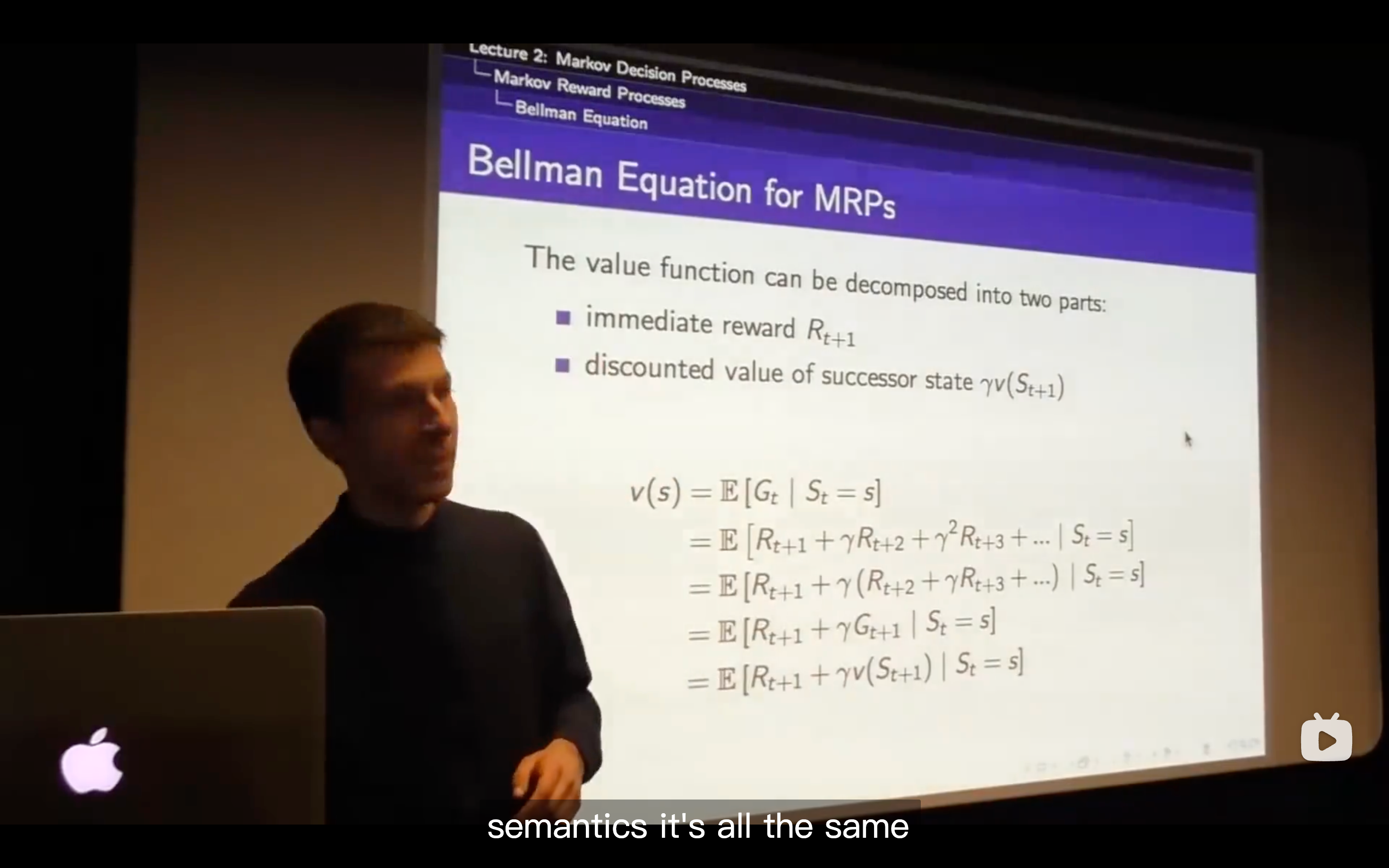
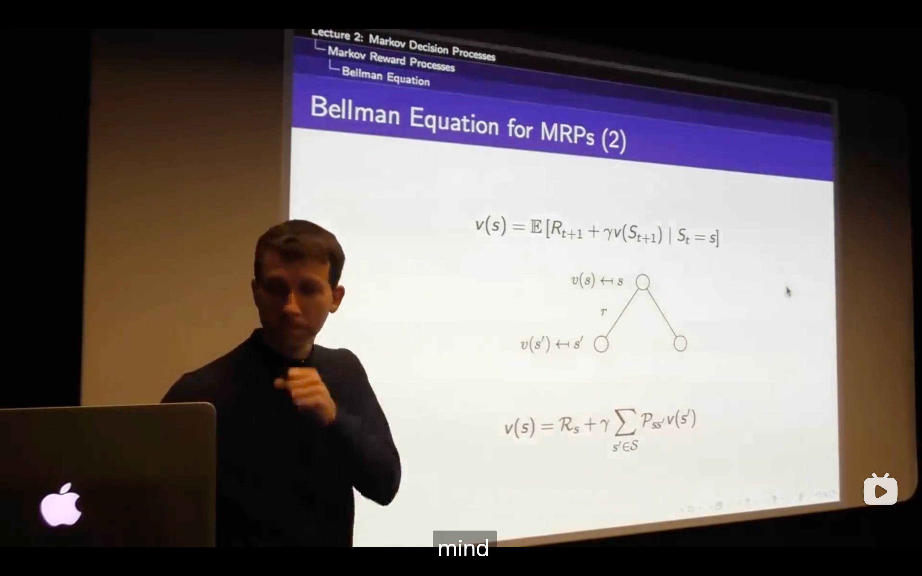
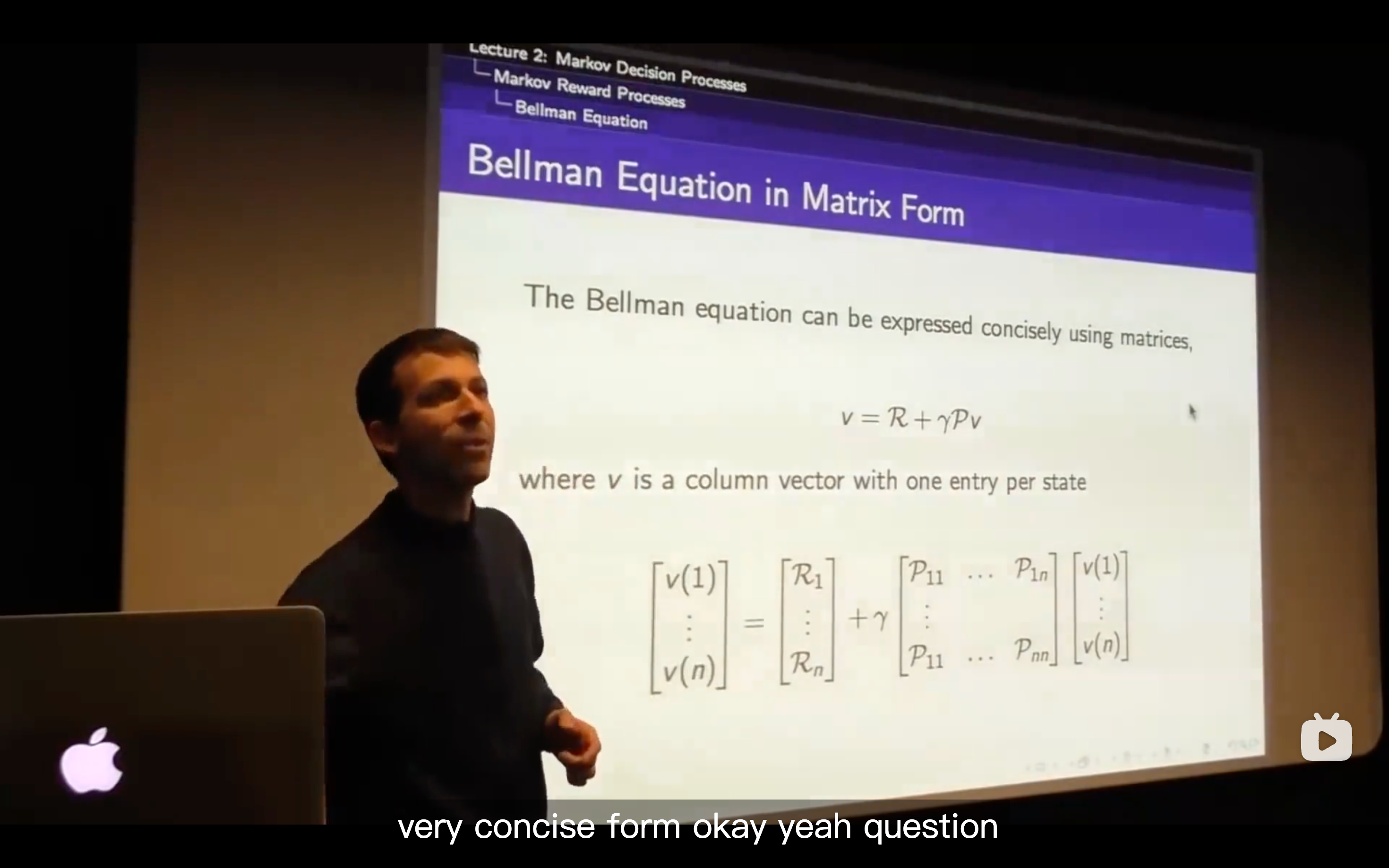
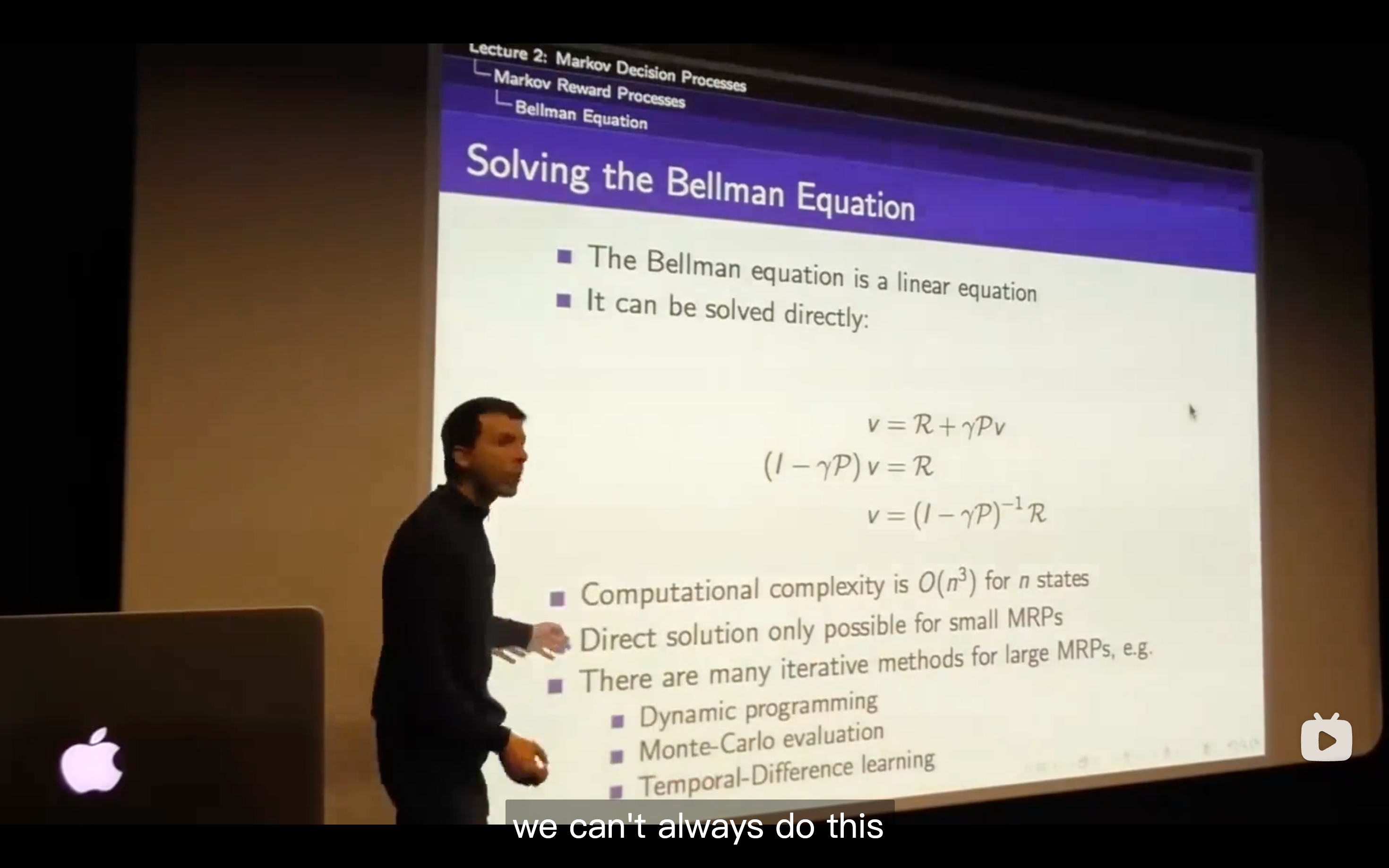
- Bellman equation may be the most fundamental relationship in RL
- It is the Markov process with some value judgement
Markov Decision Process
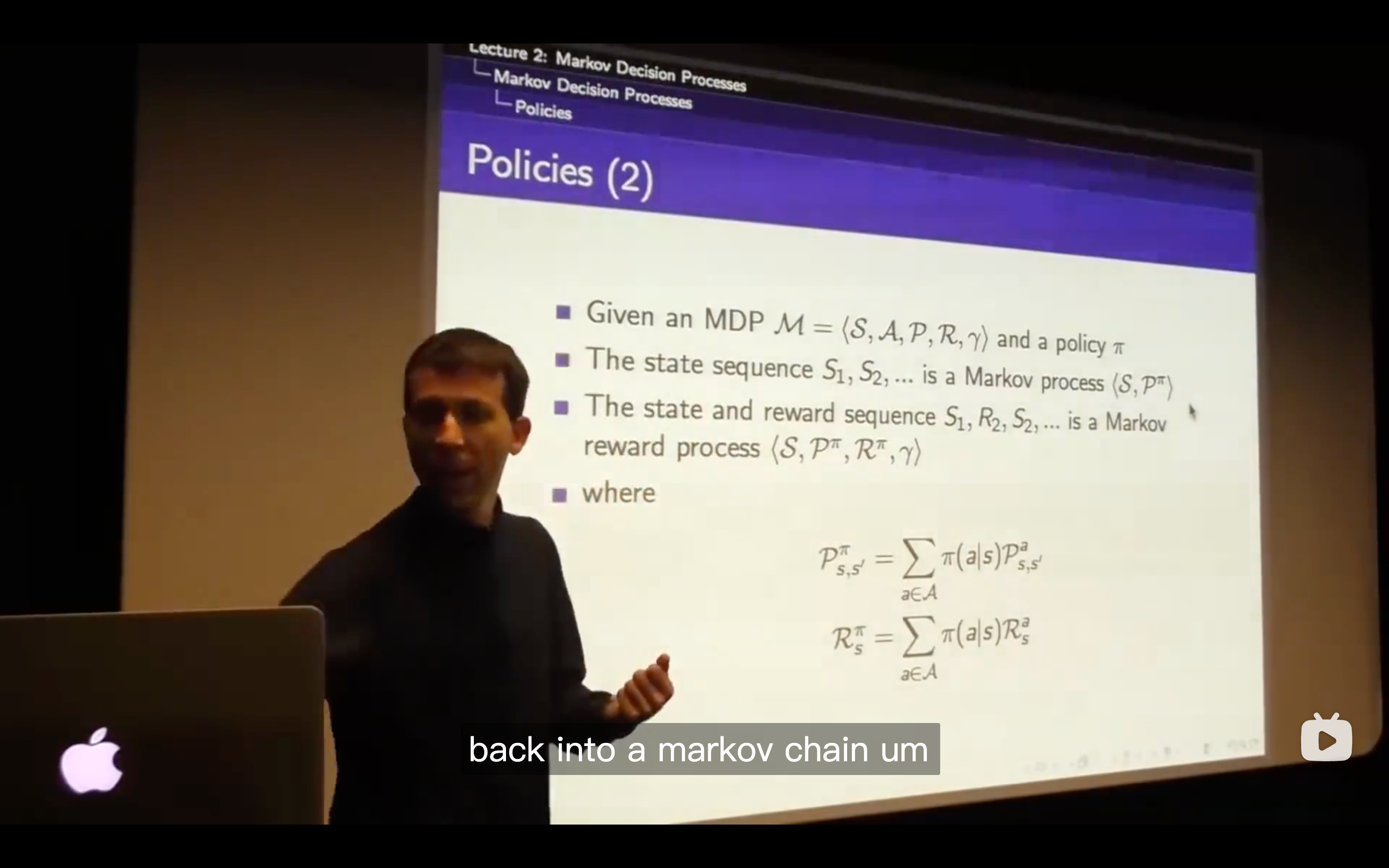
Policies
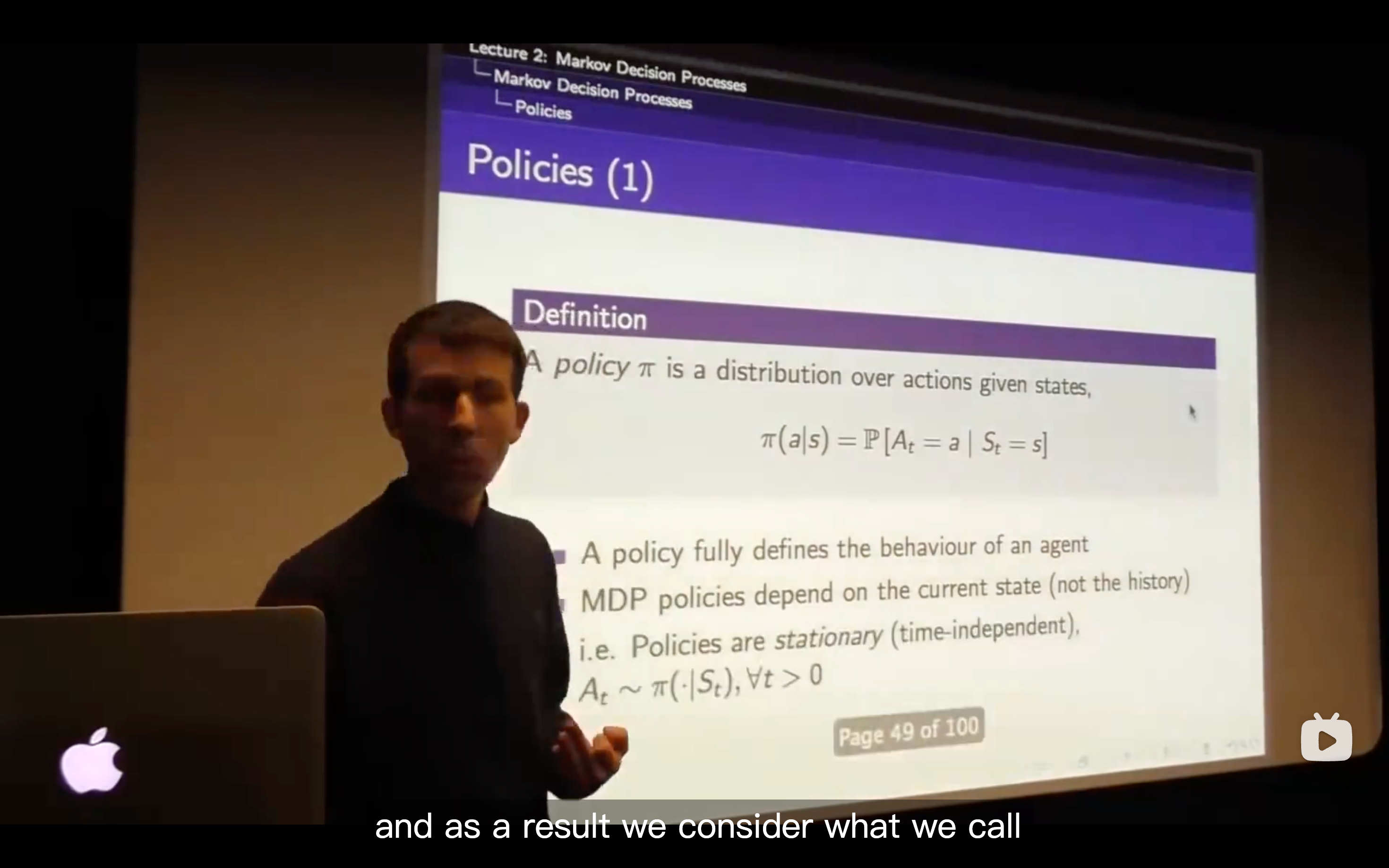
- What we want to do is maximizing the reward from now onwards that the way we' going to behave optimally.
- Our definition of state information-wise includes all the information about the expected future
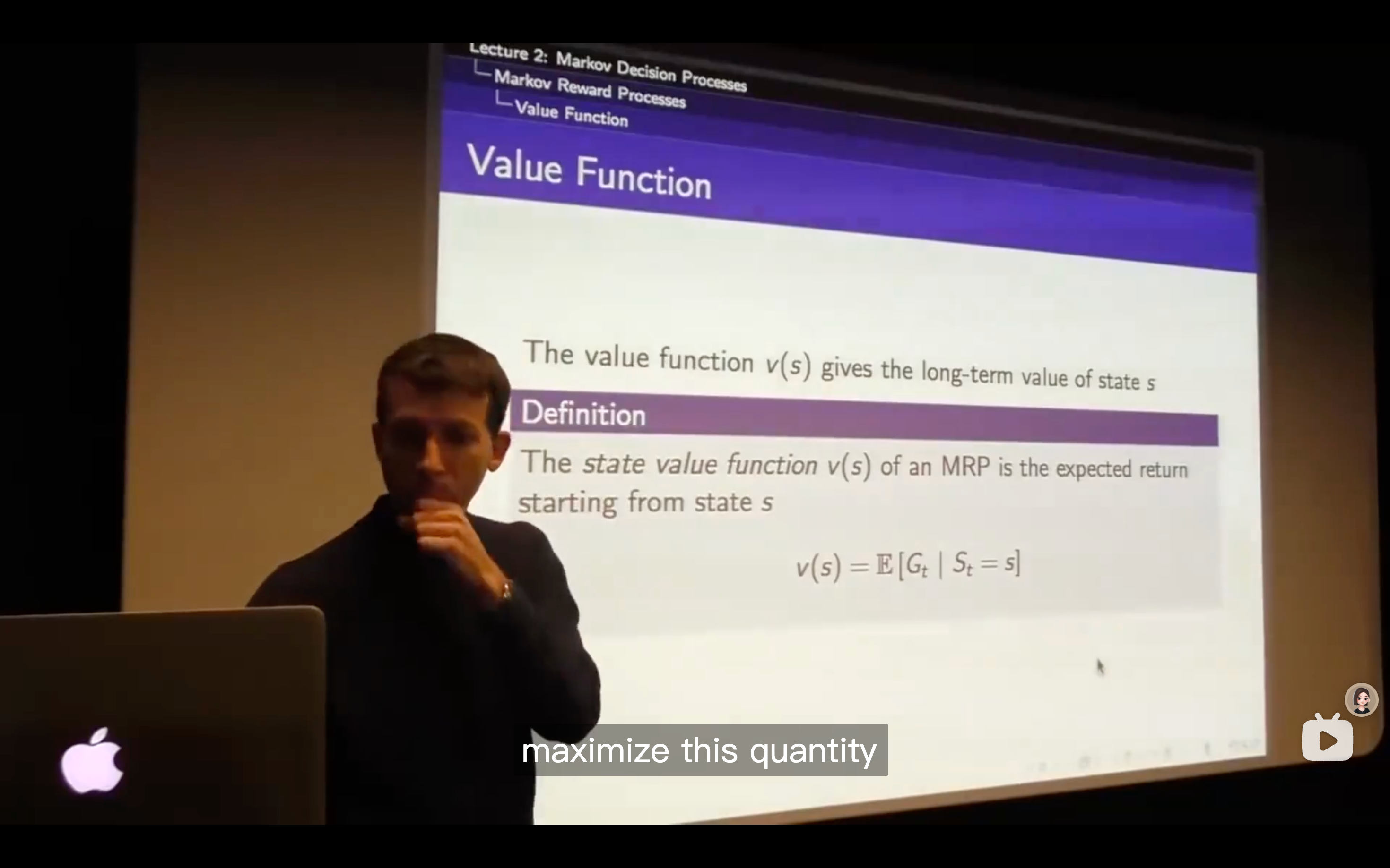
Value function
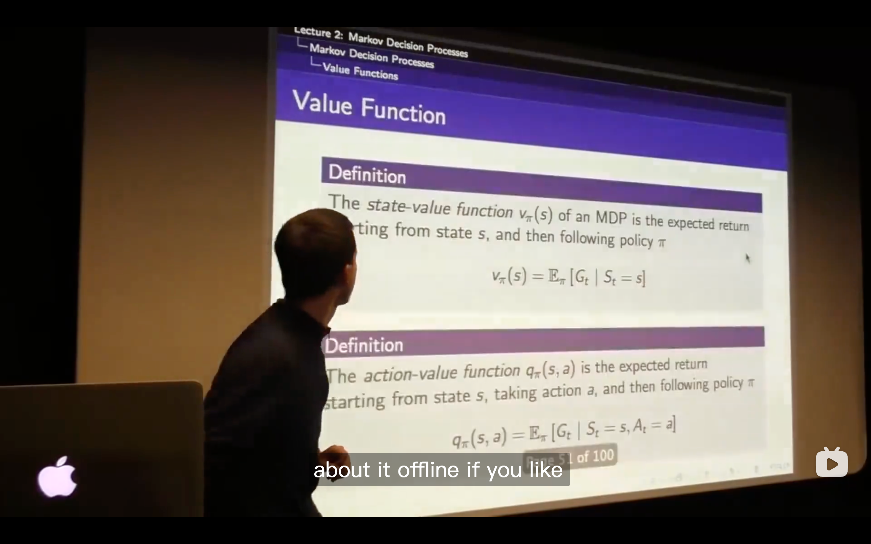
- state-value function
- The
tells us how good is it to be in state s if I'm following policy
- The
- action-value function
- state-value function
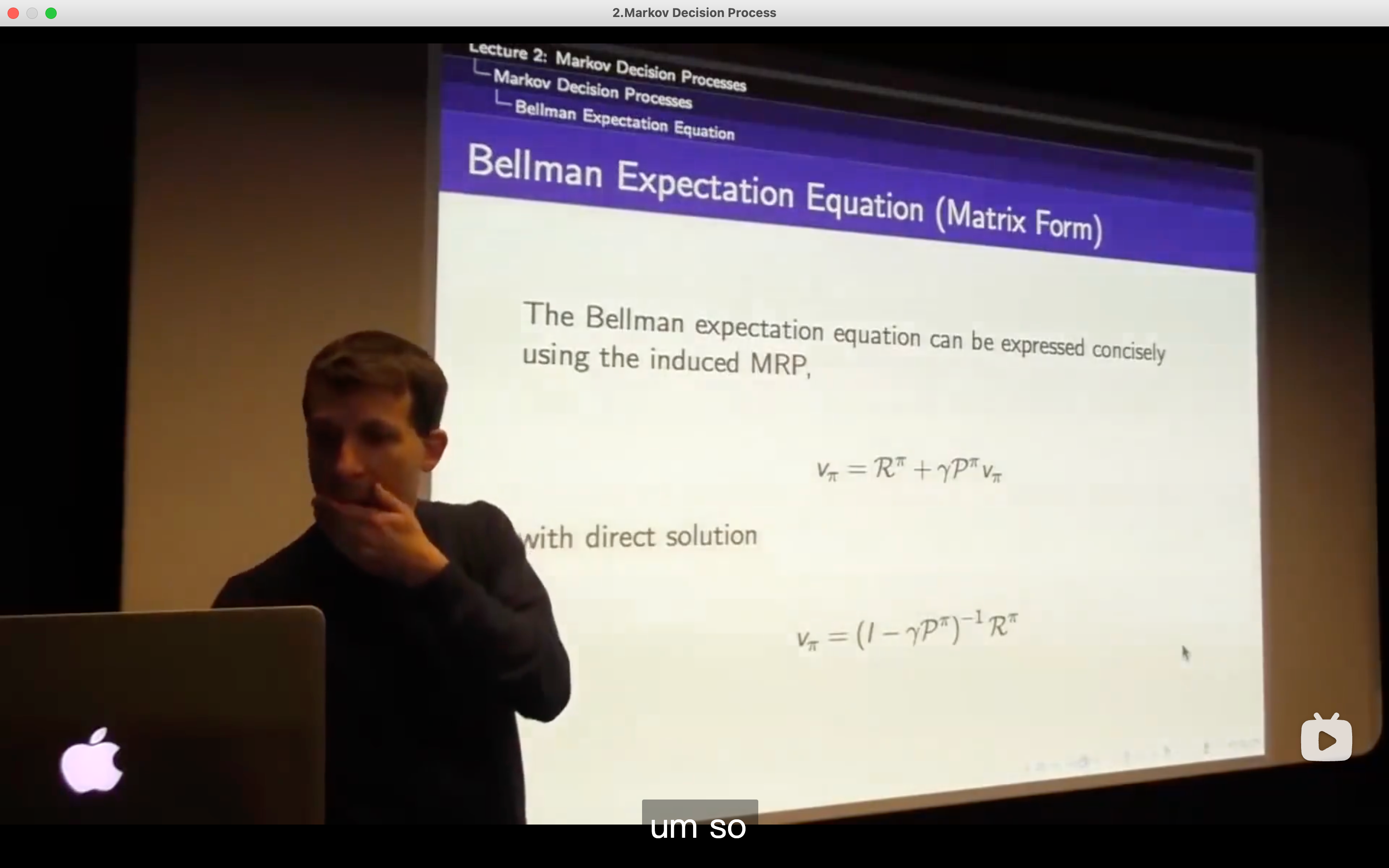
Bellman Expectation Equation
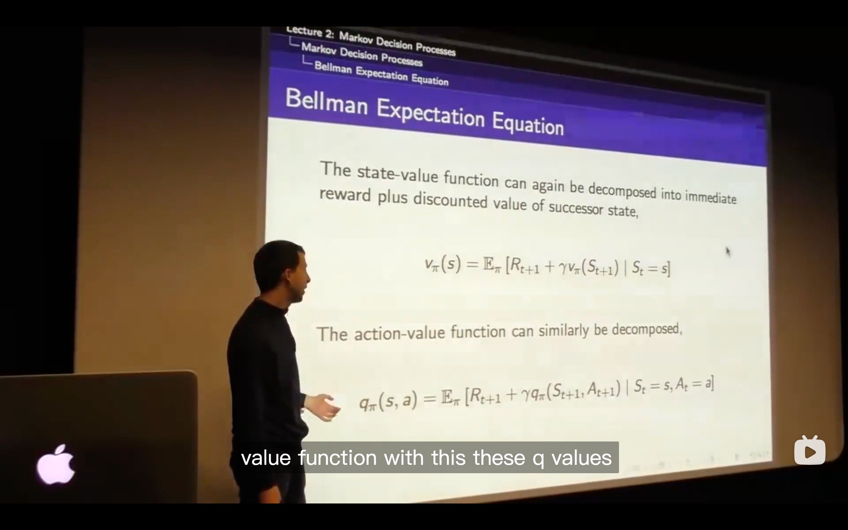
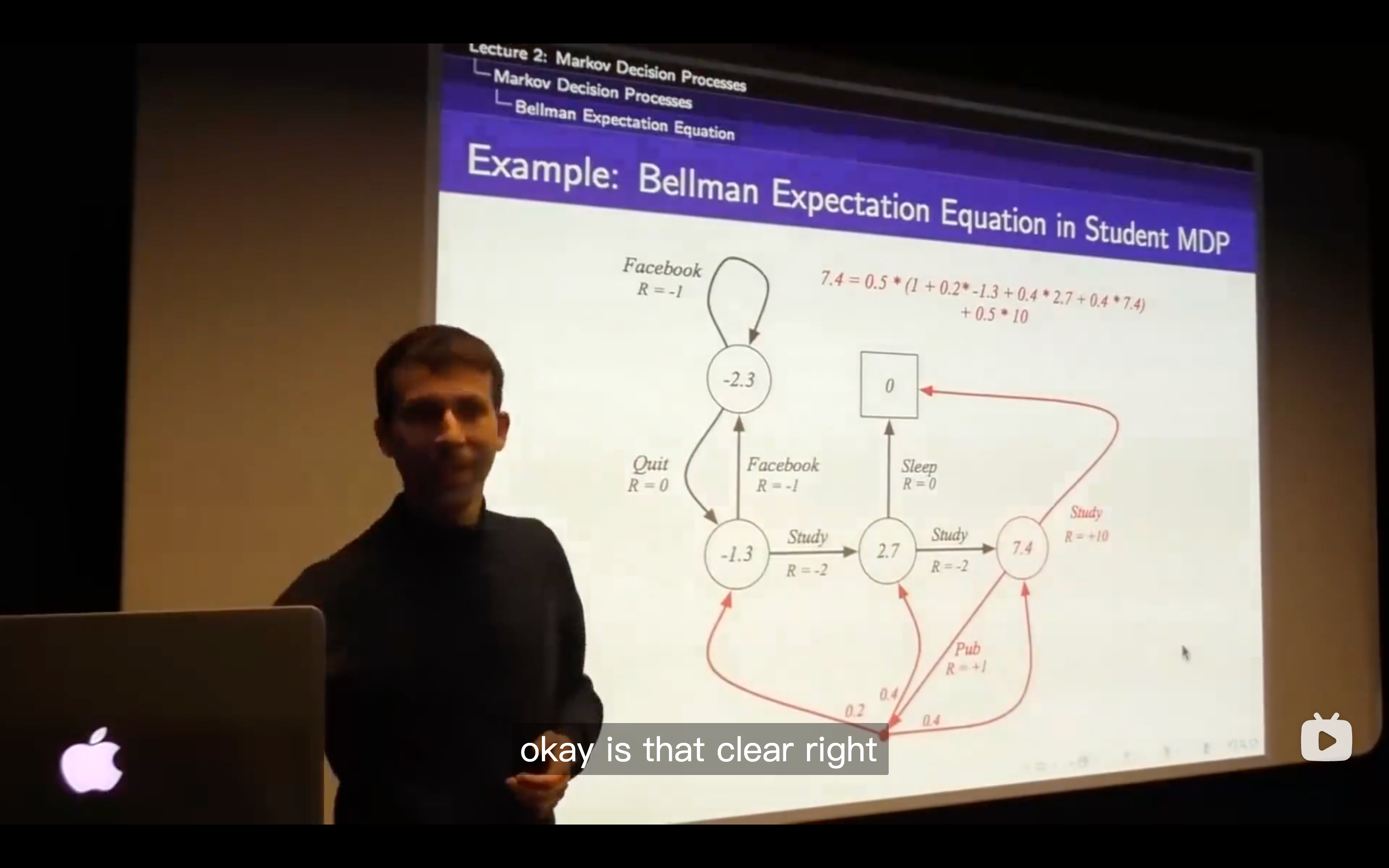
- it basically tells us now we really know how good is it to be in each one of these states you really will get 7.4 units of reward in expecation if you just behave according to this policy.
- Under the policy of this example, we do everything with the probability of 50 percent.
- In this map, the reward does depend on the action you take
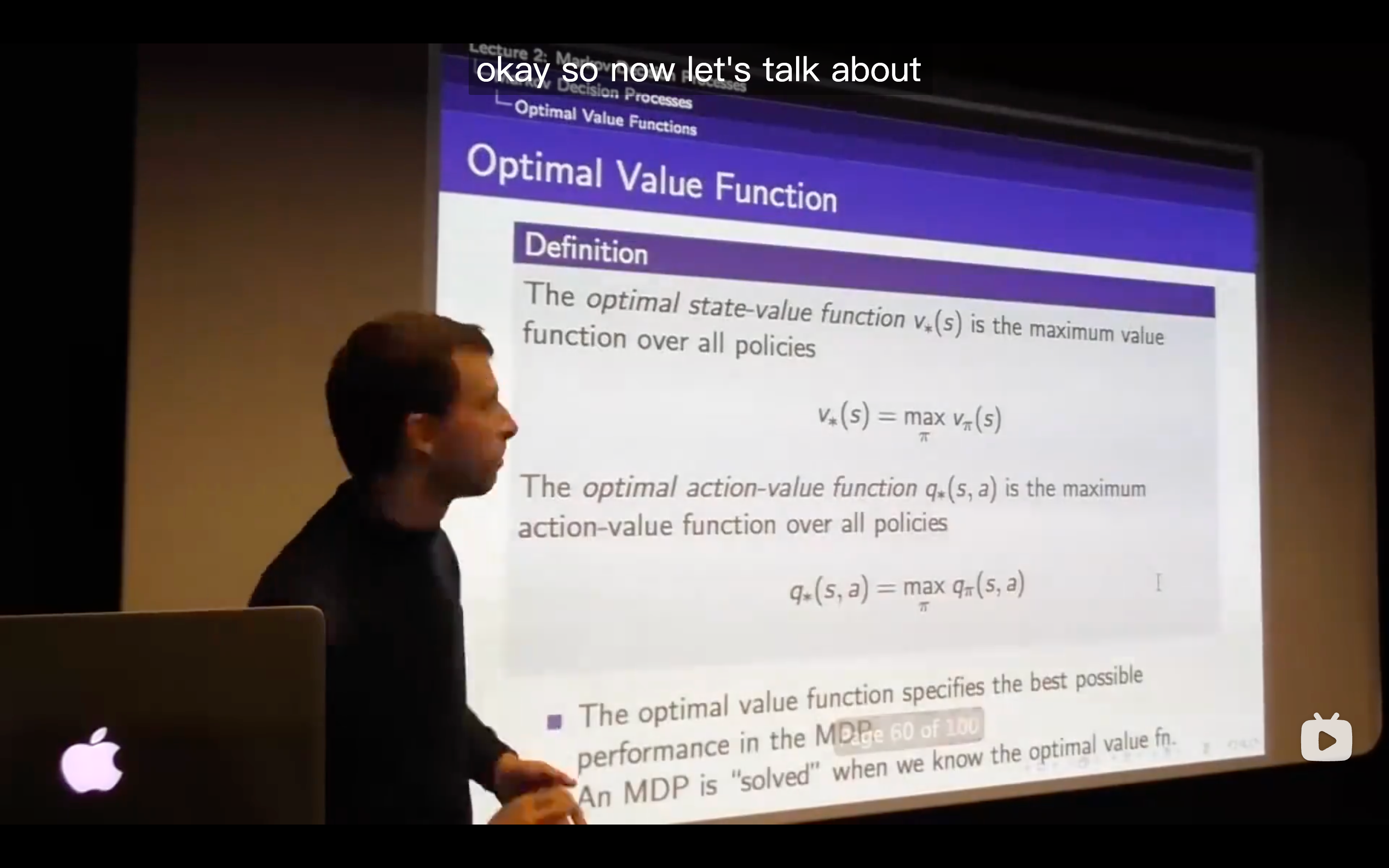
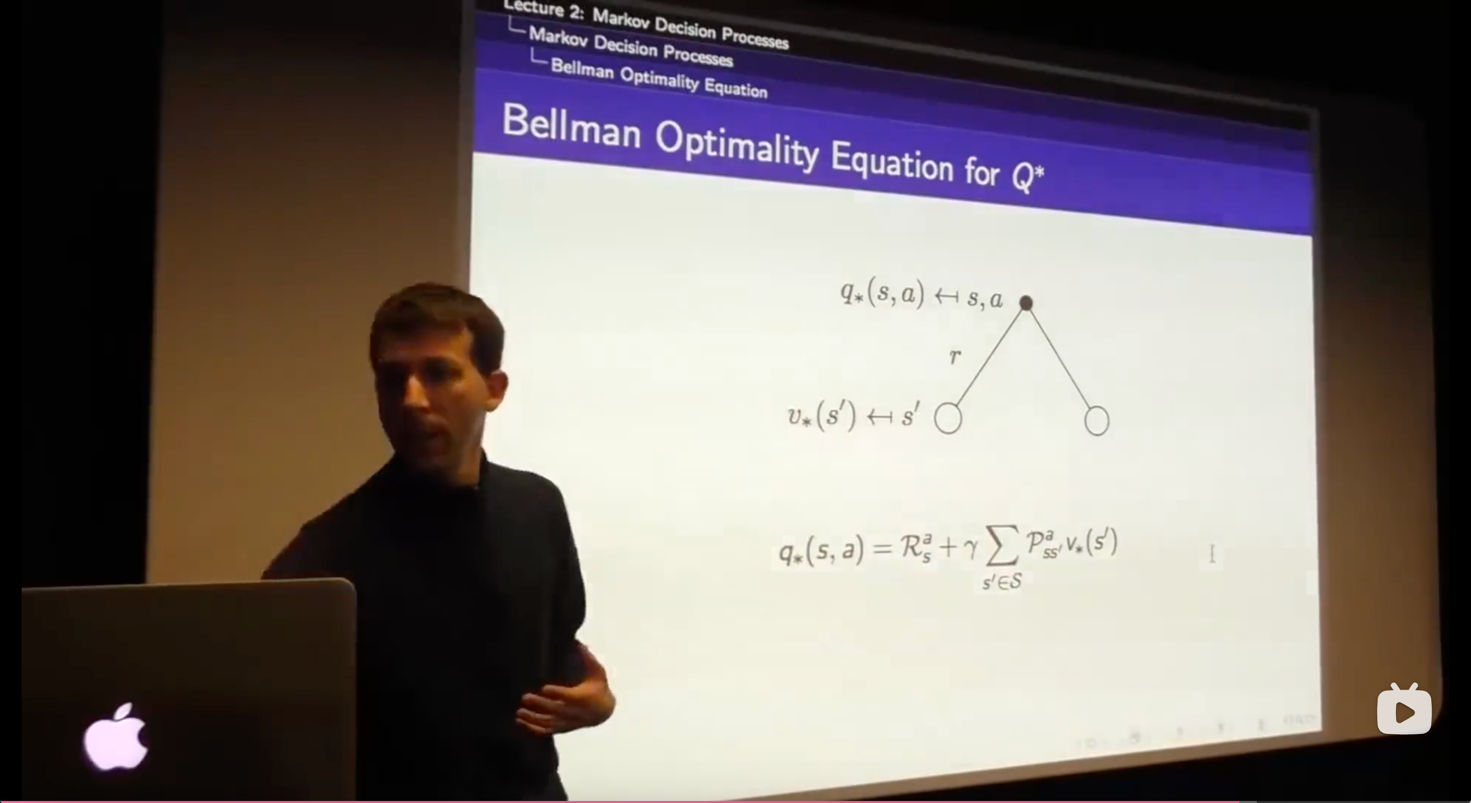
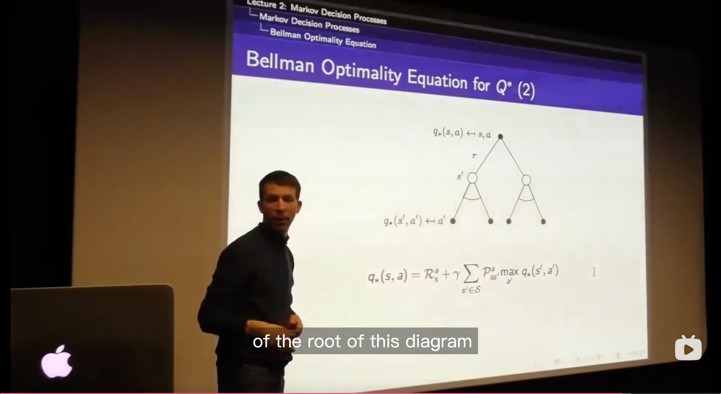
Optimal Value Function
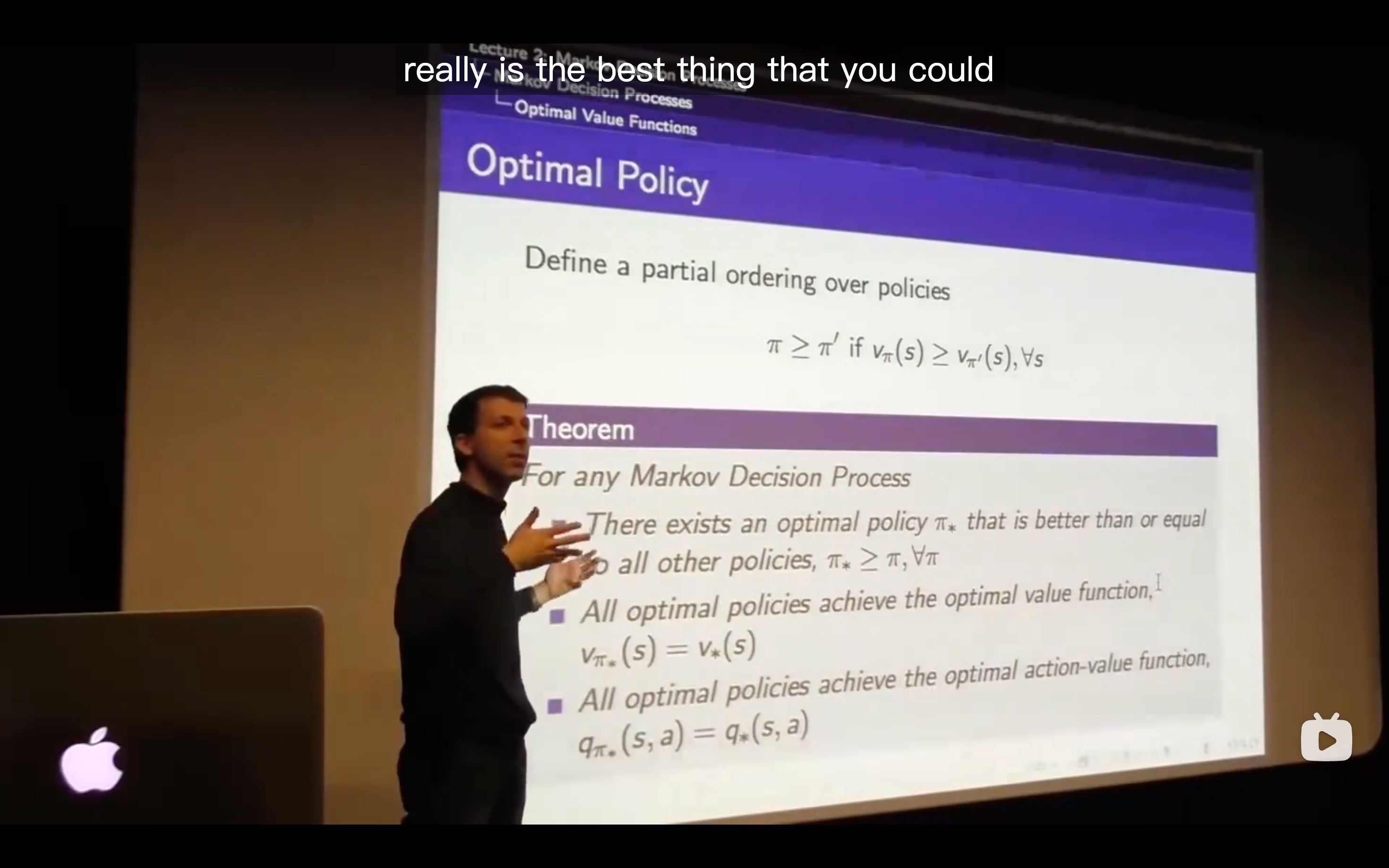
Optimal Policy
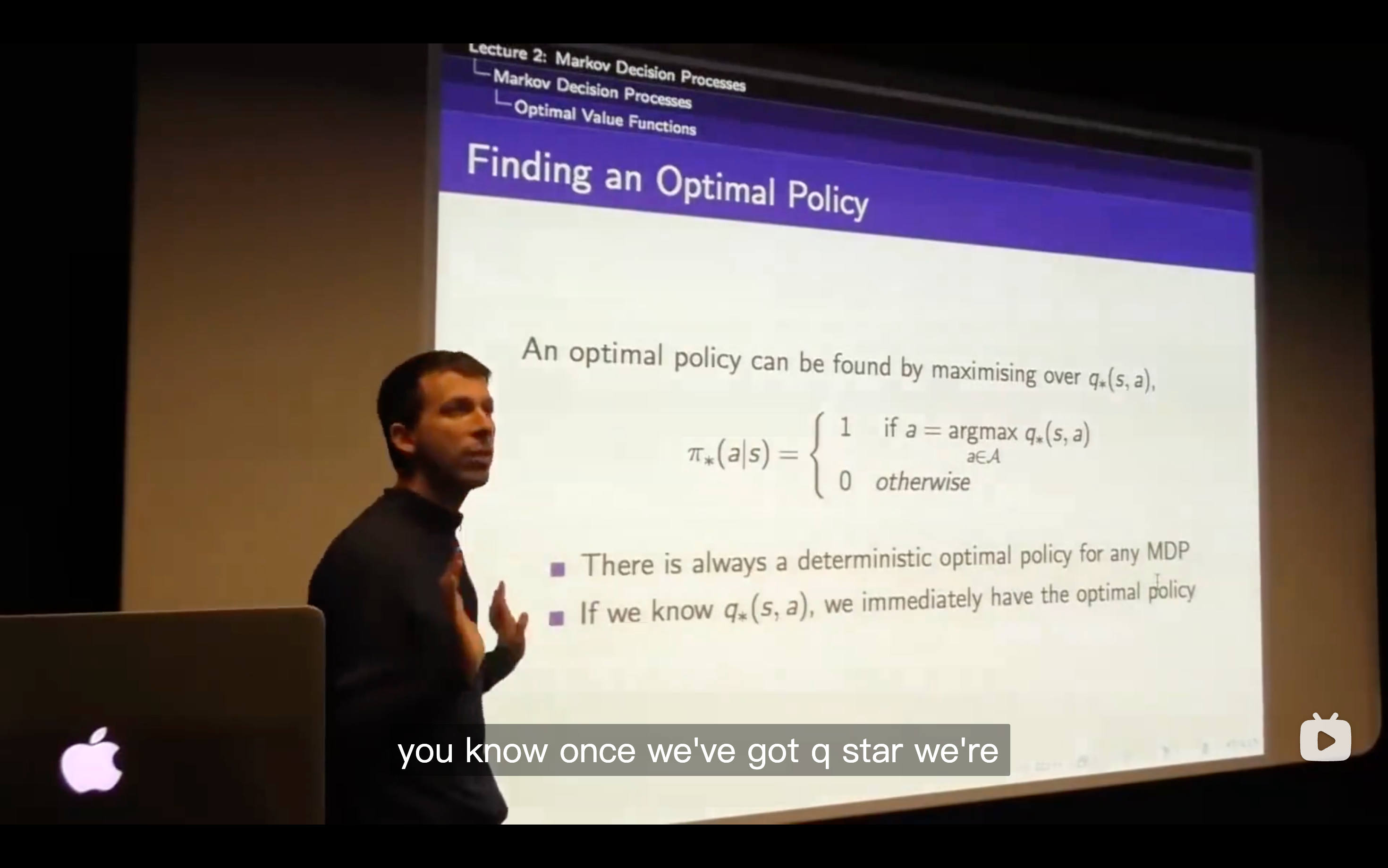
- An optimal policy can be found by maximising over action-value function.
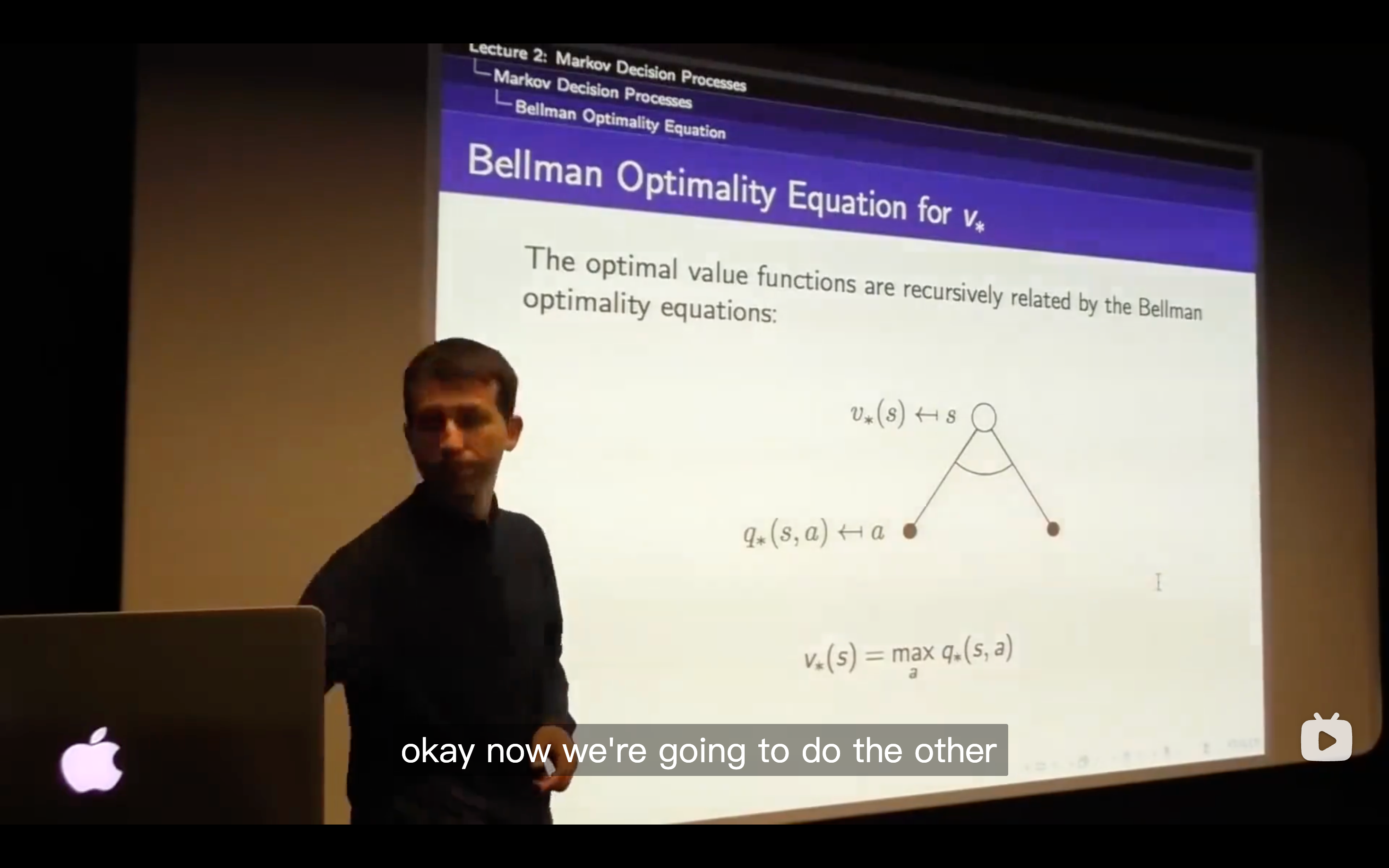
The max of the q values can be achieved by picking up the max of values of each of the actions that you can take from that state.
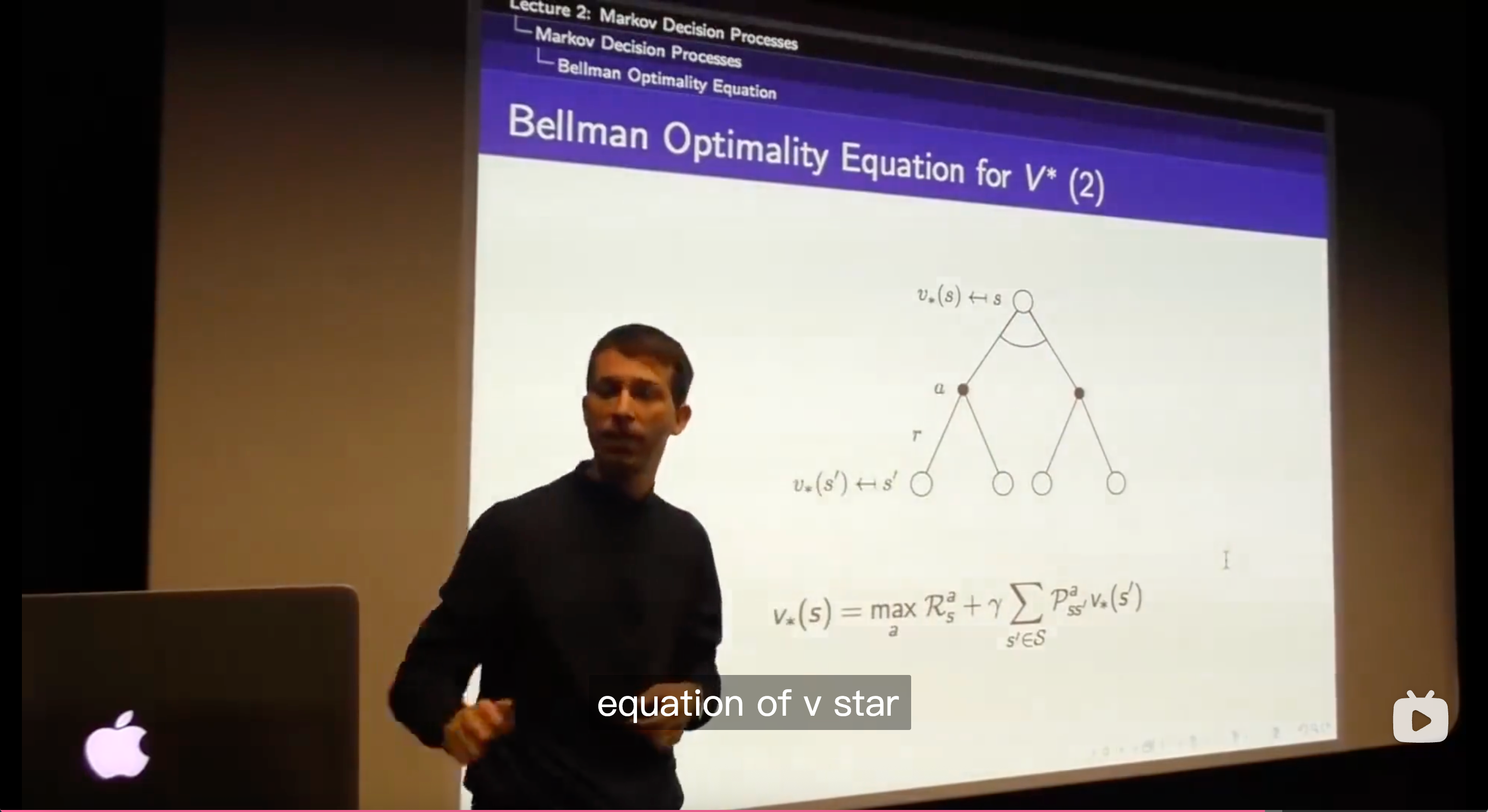
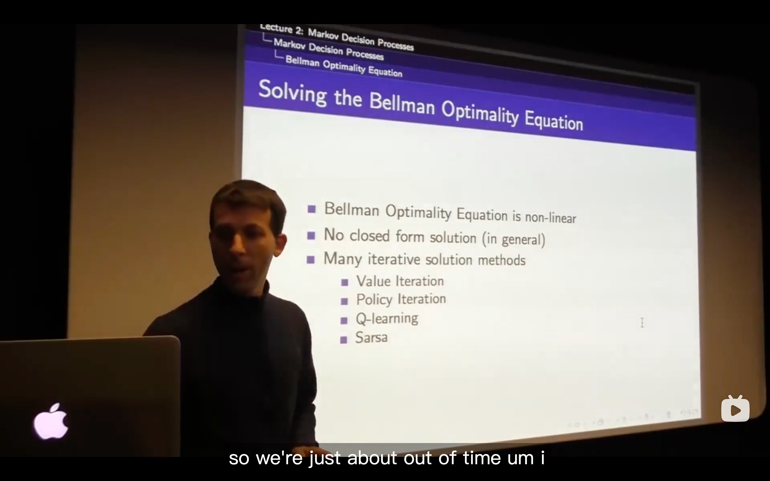
- All you need to do is to figure out how do I behave optimally for one step, and the way you behave optimally for one step is to maximize over those optimal values functions in the places you might end up in.
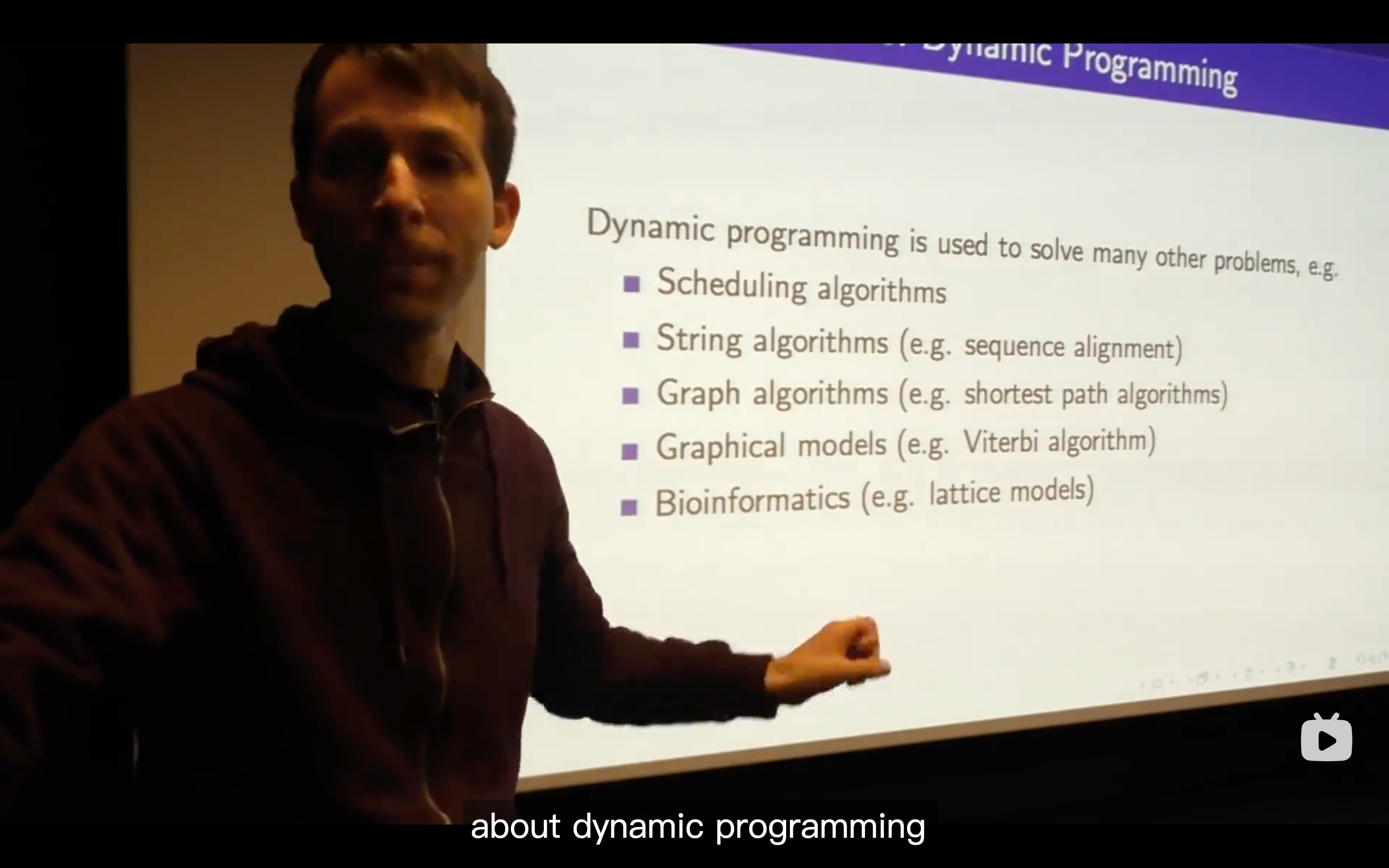
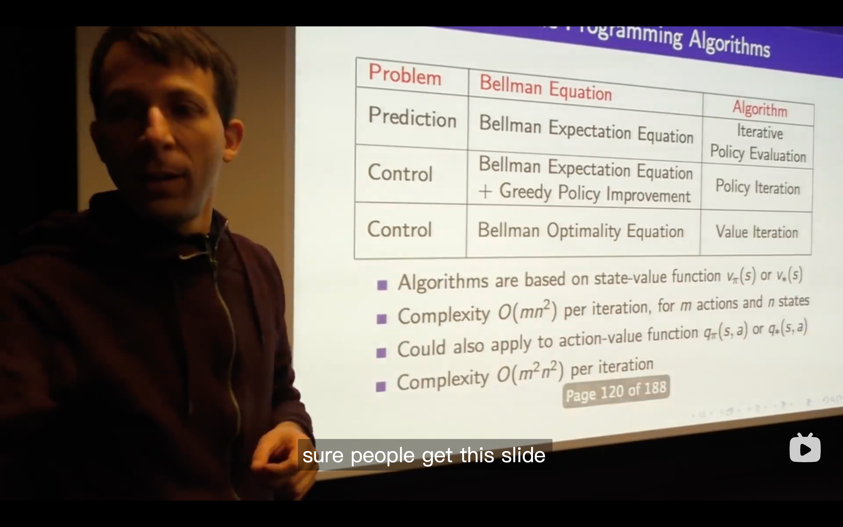
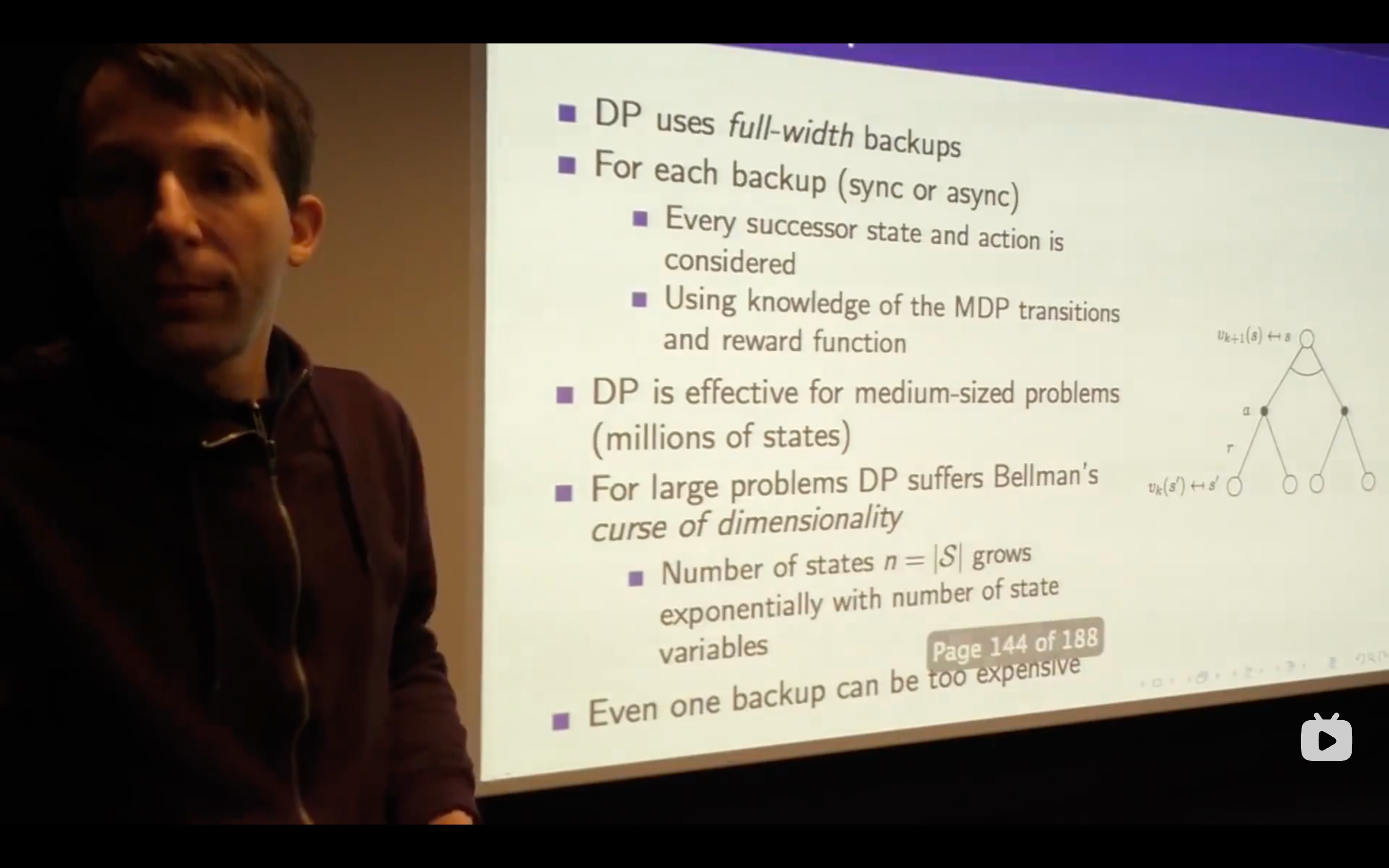
Lecture3: Planning by Dynamic Programming
Intro
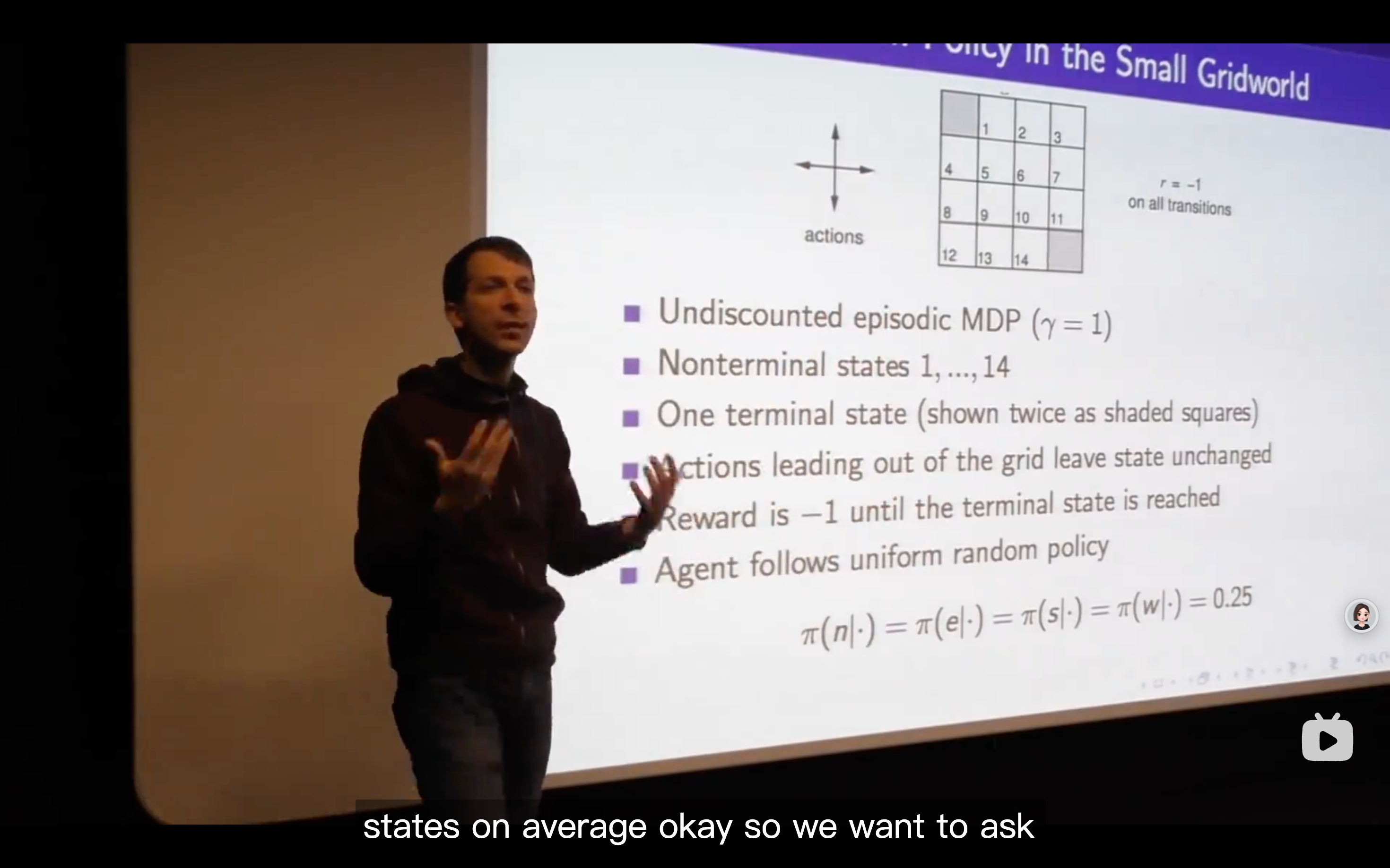
Planning in an MDP
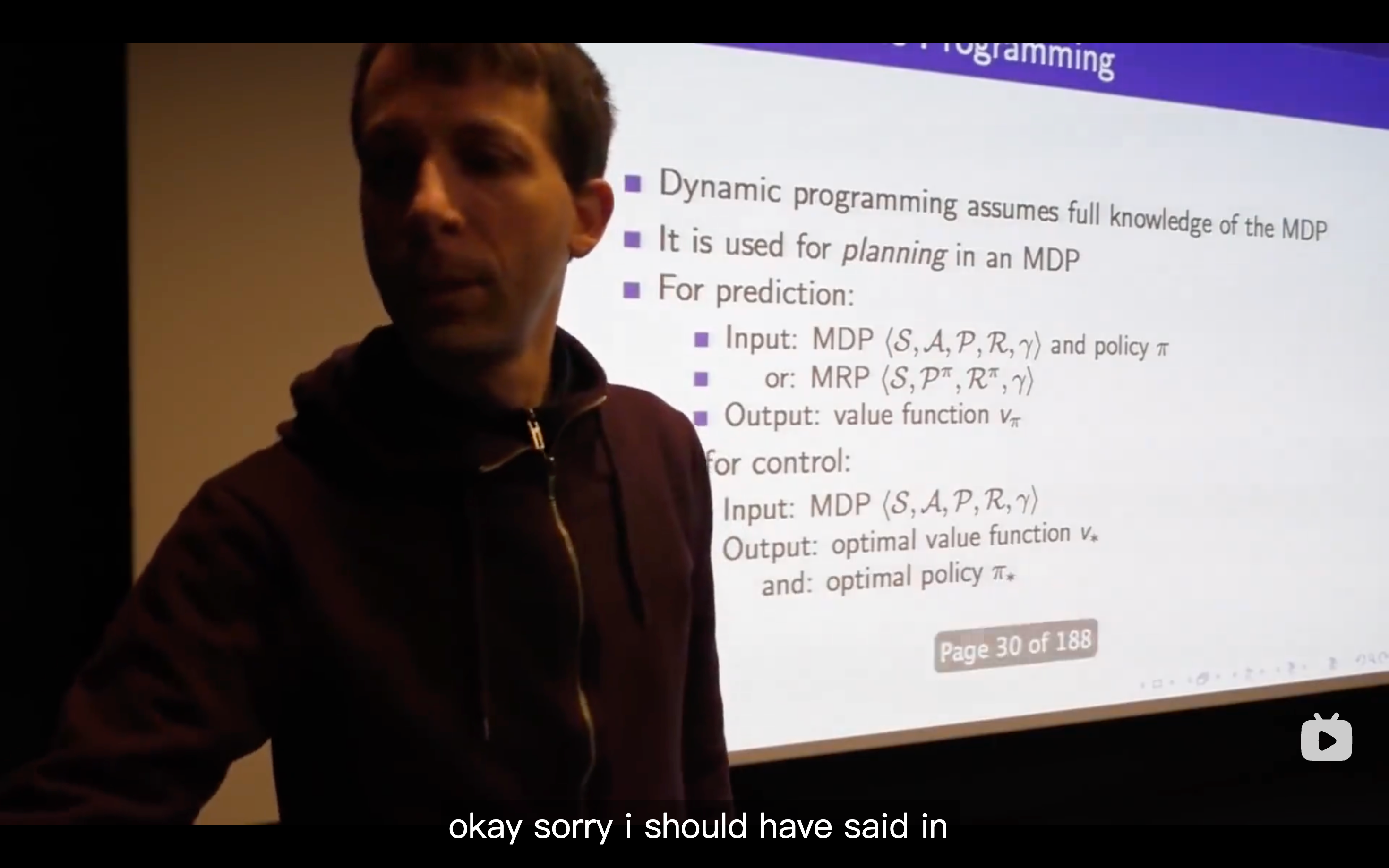
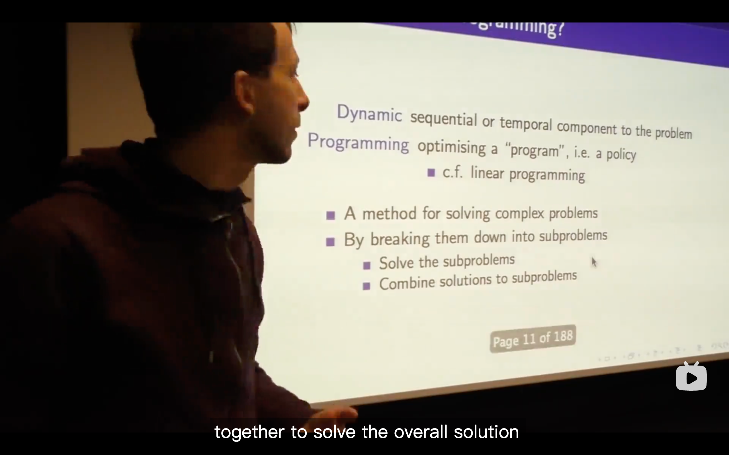
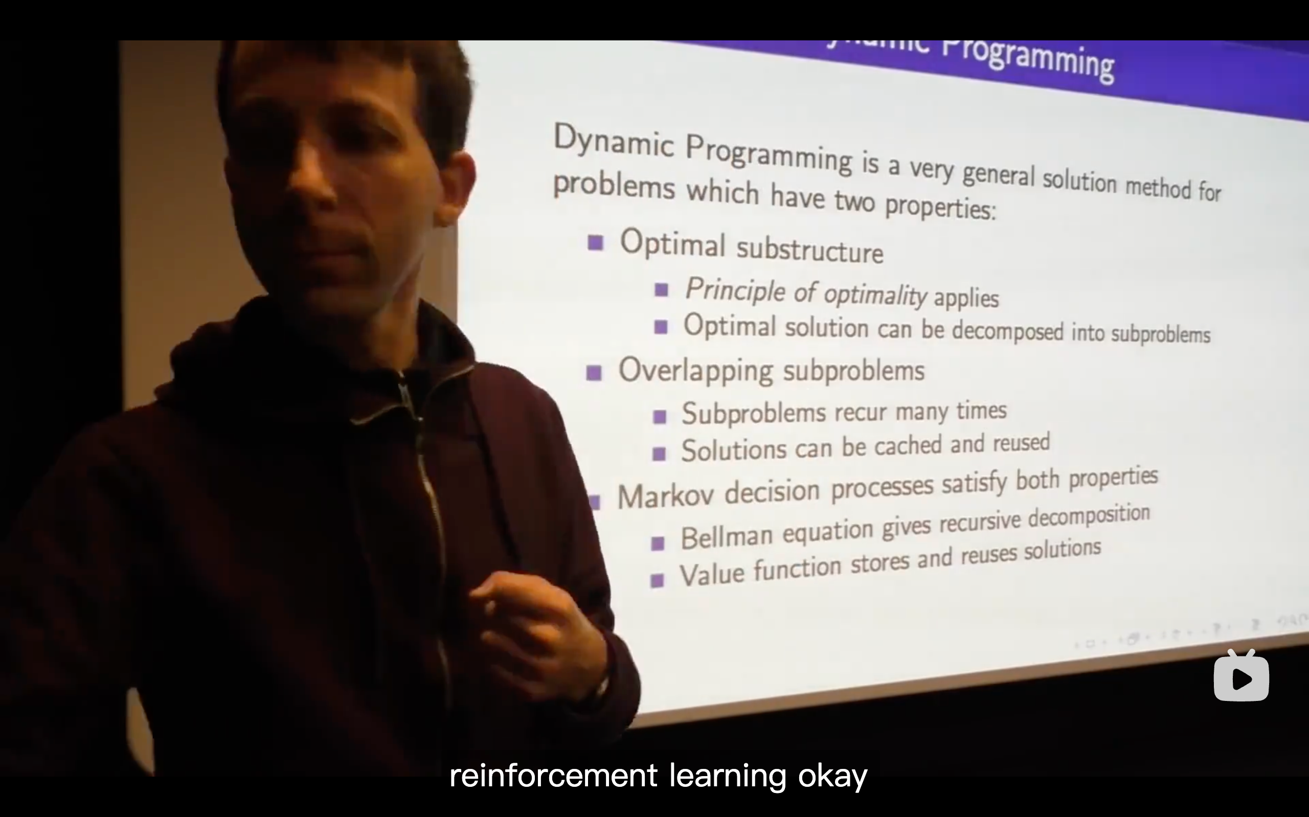
What's a Dynamic Programming solving?
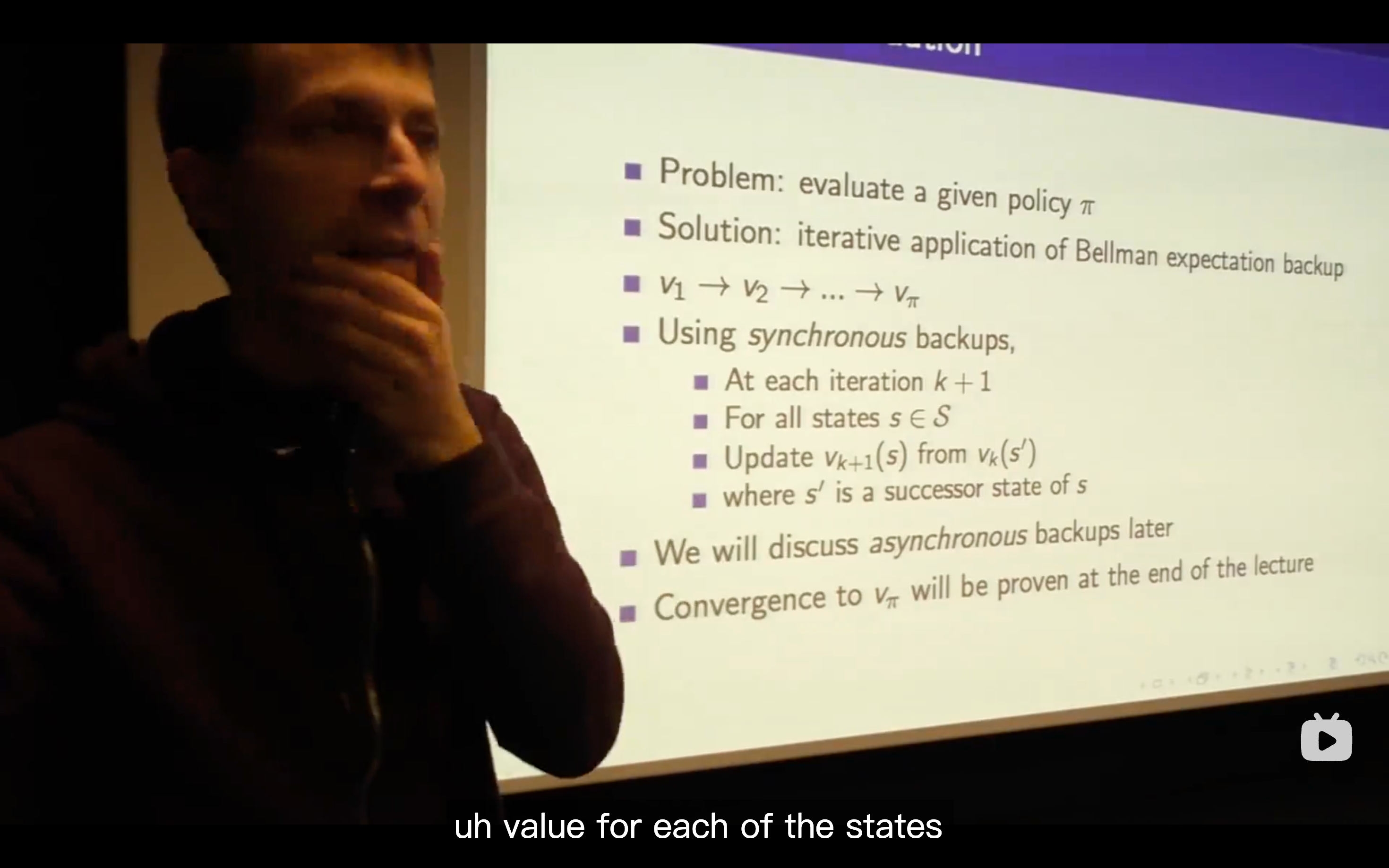
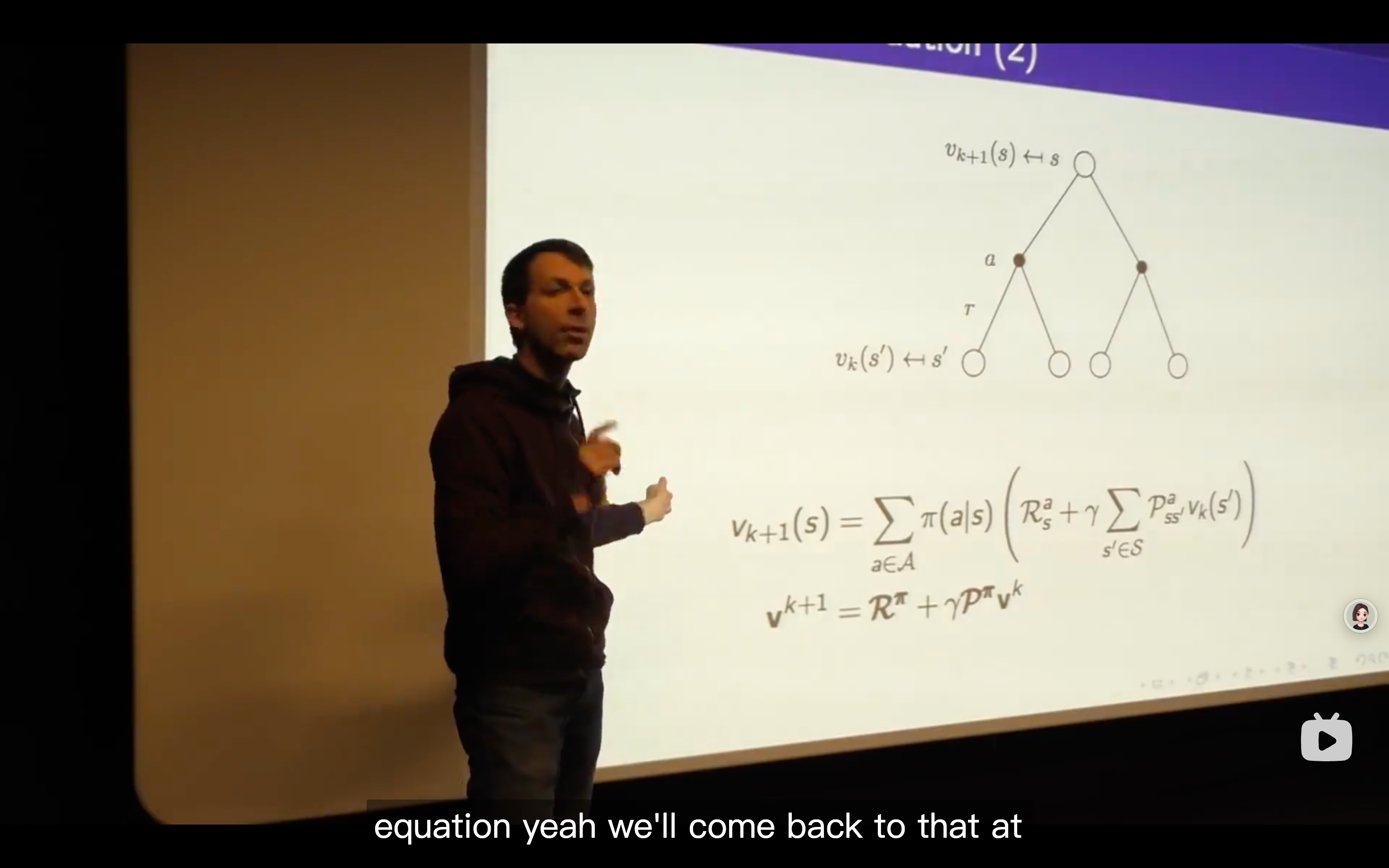
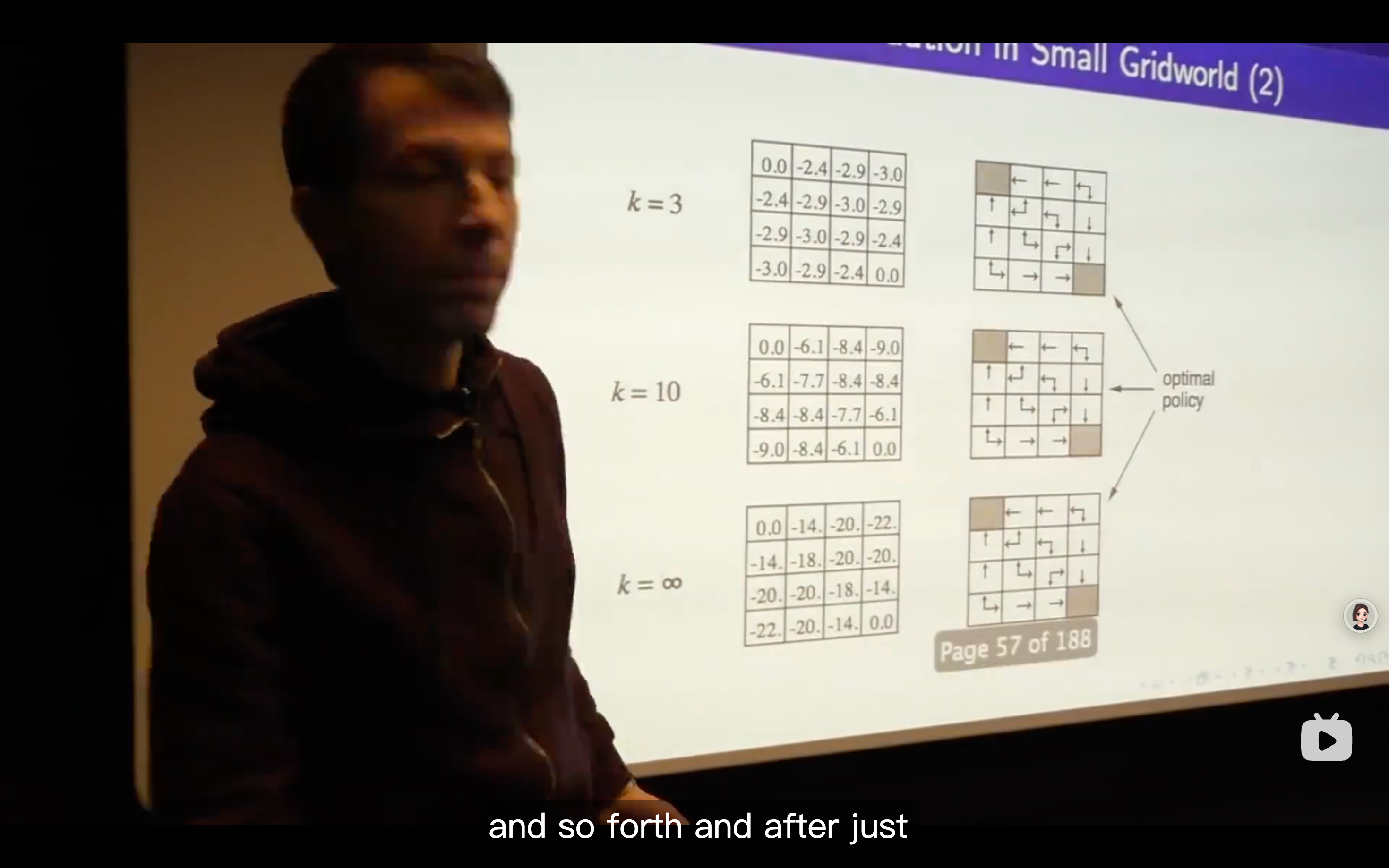
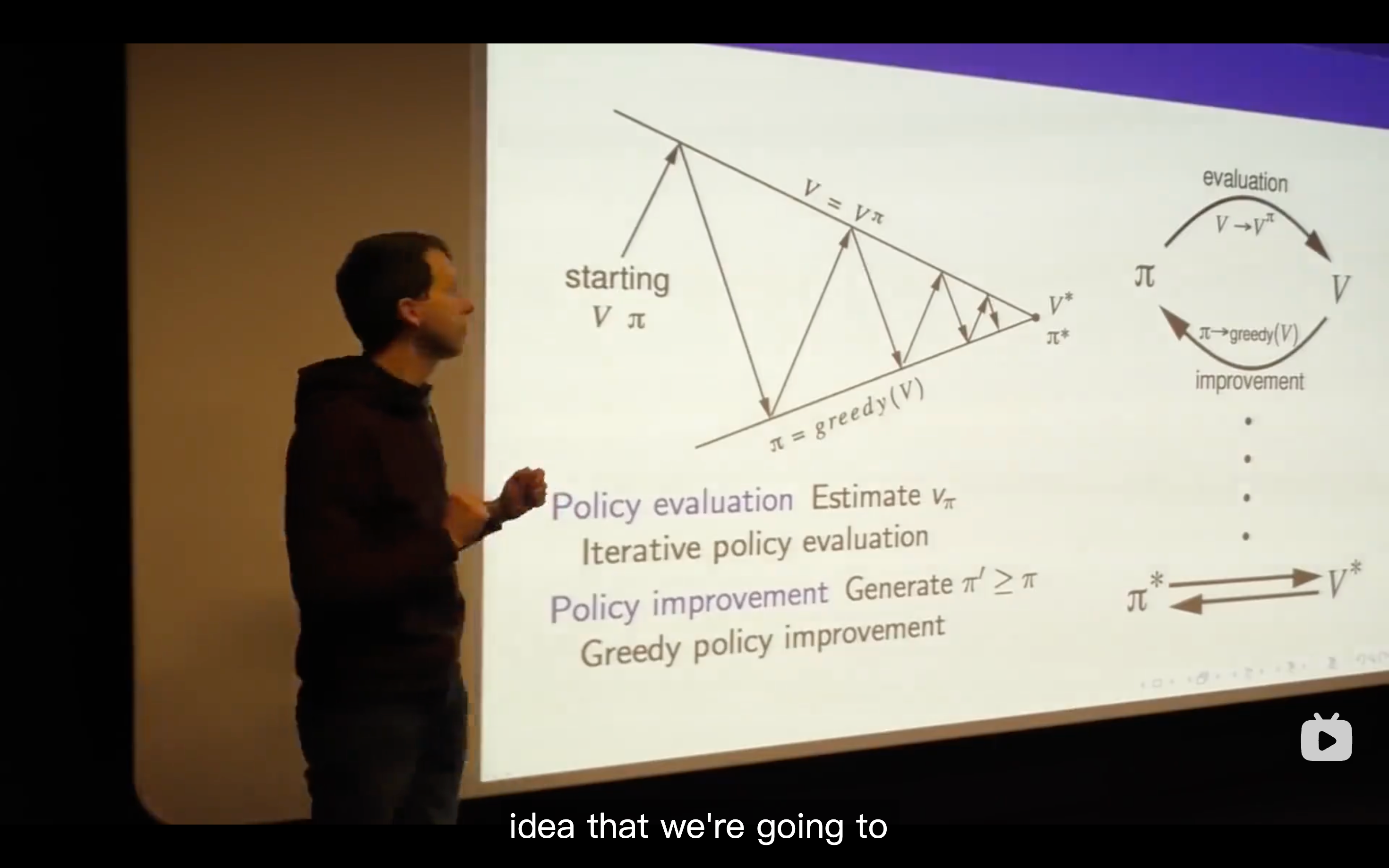
Policy Evaluation

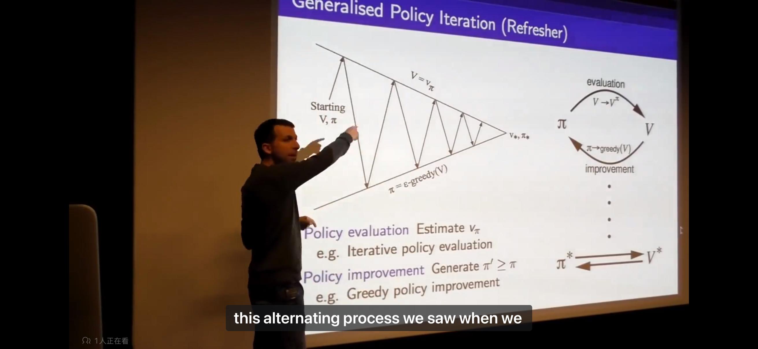
Policy Iteration
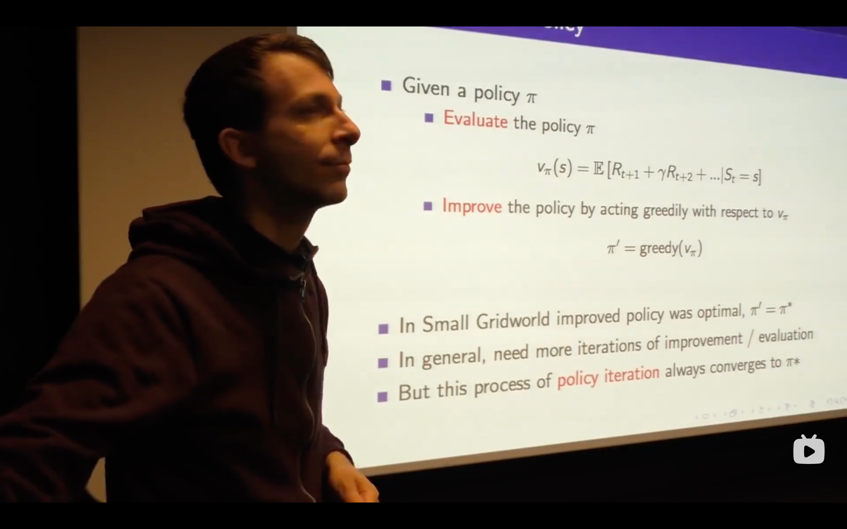
- There's always at least one deterministic optimal policy for any MDP, so it's sufficient to actually search over deterministic policies only when youre looking for the optimal policy.
- No matter where you start for any value and any policy, you will always end up with the optimal value function and the optimal policy.
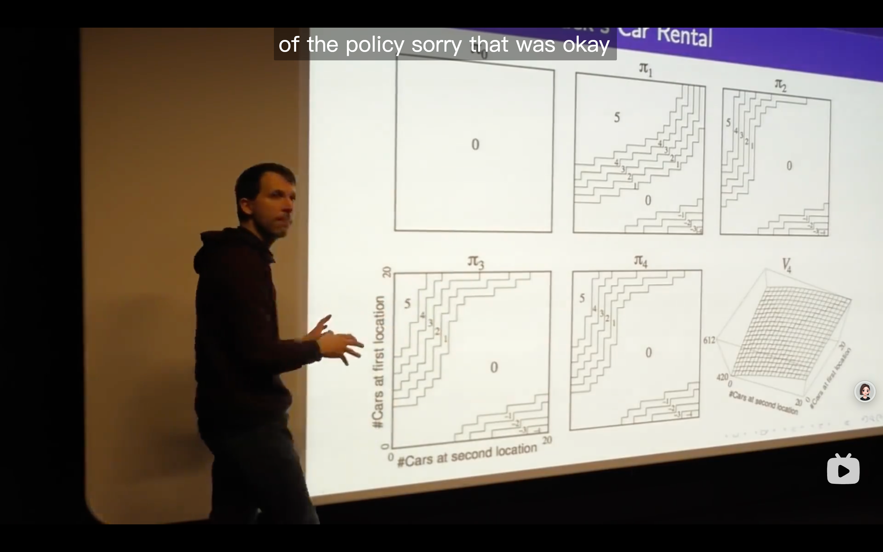
- This is a contour map of this policy, the density of these grid worlds represent the speed of value changing. The more, the faster.
- evaluate the policy, then come up with a new surface( which is in the representation of value function in a two dimensional axes.)
- There's no cost in moving a car in this example.
- The
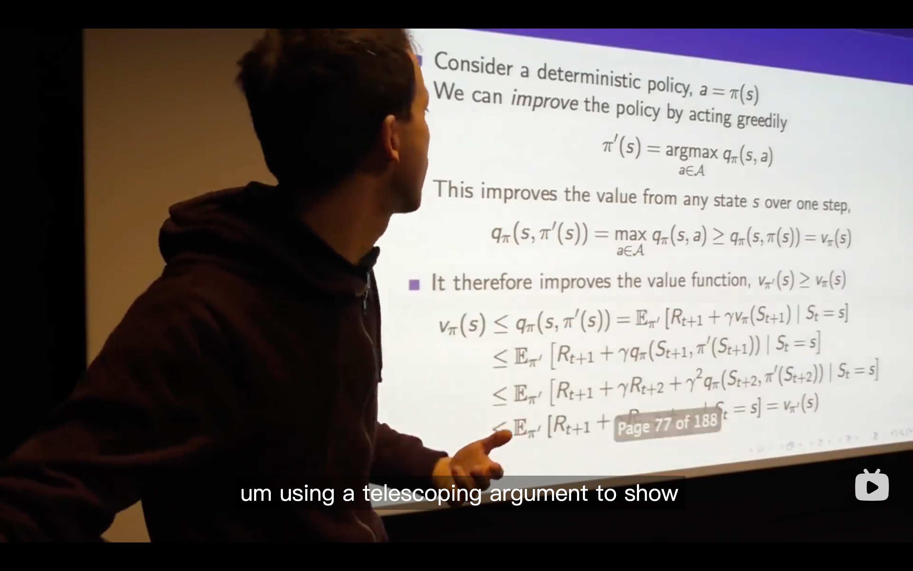
is just the immediate reward plus the value of the next, that's what we act greedily. - Let's not worry yet about what happens after that, let's just consider one step and see whether we get more value over one step.
- The max over the
has to be at least greater than equal to one particular so the max over all actions has to be at least as good as one particular action that we could plug in which is what the one we were choosing before. - So all of this that's a long-winded way to say that the value function improves over one step at least that if we just take our
for one step, we'll get at least as much reward as the policy we started with. - So we don't make things worse ever, we always make things at least make them better, (though) we haven't yet said that this is guaranteed to keep getting better or to reach the optimal value.
- Being greedy doesn't mean that we only look at one step of immediate reward, instead, it means that we look at the best action we can take if we optimize over all actions we can do for one step, and then look at our value function which summarizes the whole future —— all future rewards we're going to get going into the future but under our previous policy.
- There's always at least one deterministic optimal policy for any MDP, so it's sufficient to actually search over deterministic policies only when youre looking for the optimal policy.
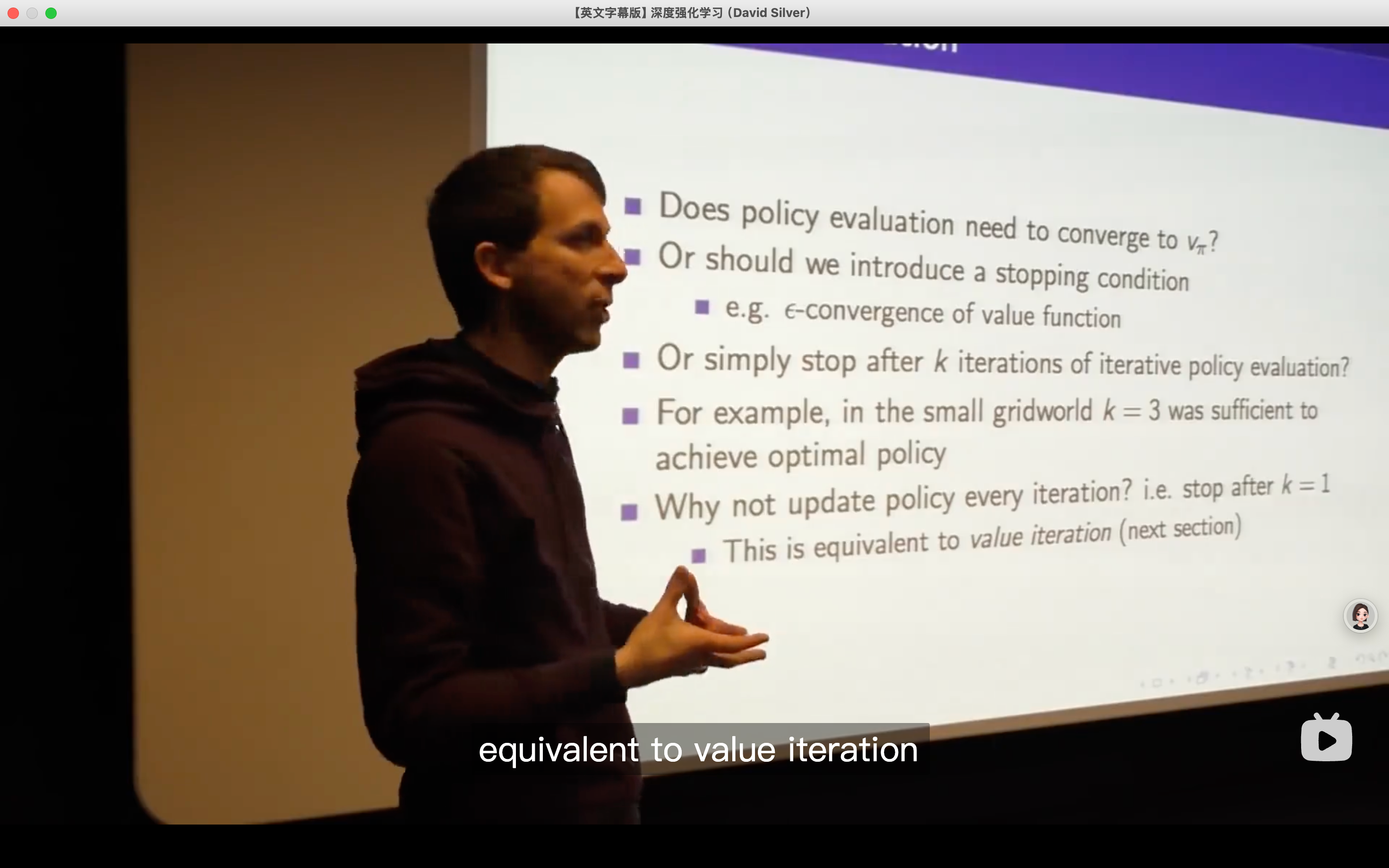
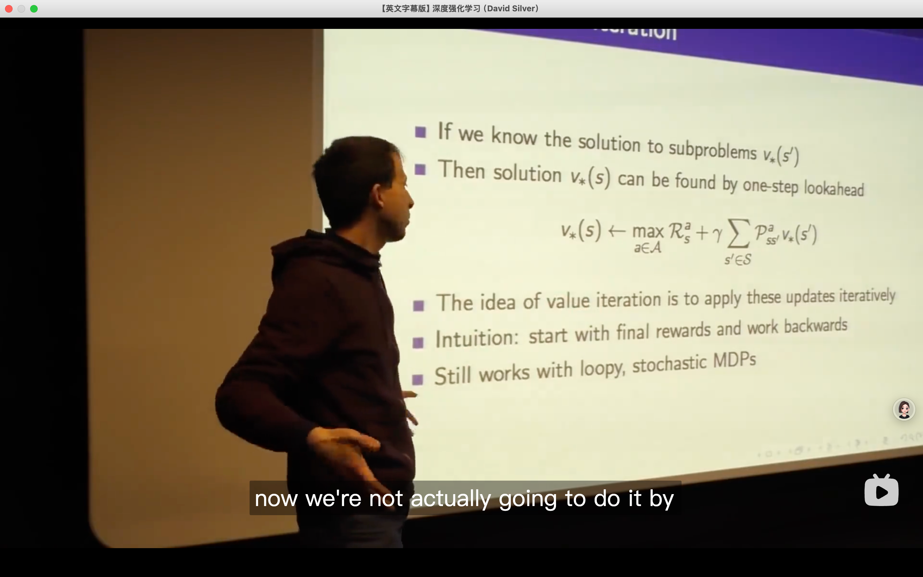
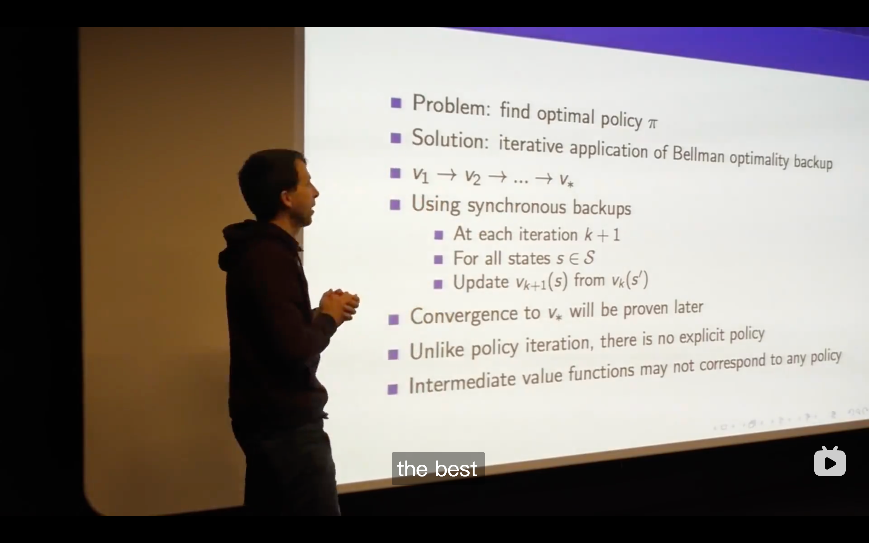
Value Iteration
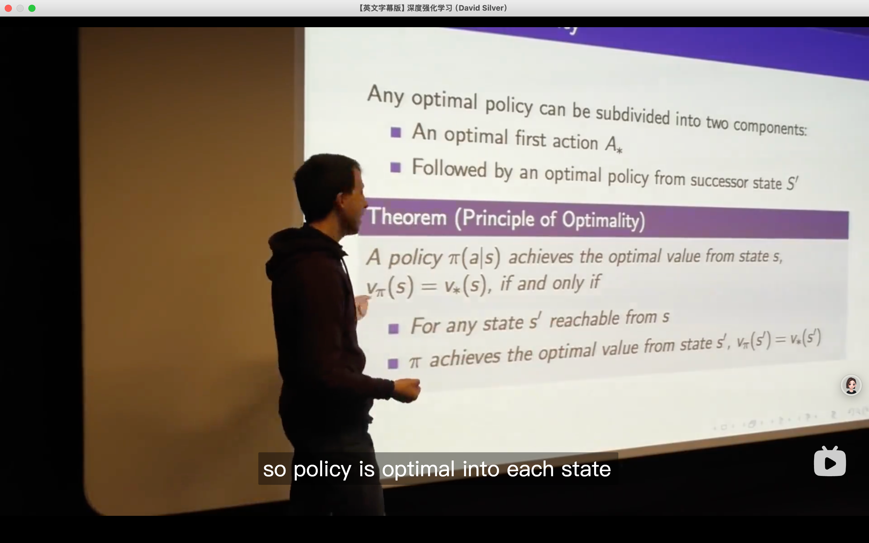
- So if my first action is optimal and then after that I follow an optimal policy from wherever I end up then we can say that the overall behavior is optimal。
Artificial Intelligence: Foundations of Computational Agents -- Value Iteration Demonstration
- So if my first action is optimal and then after that I follow an optimal policy from wherever I end up then we can say that the overall behavior is optimal。
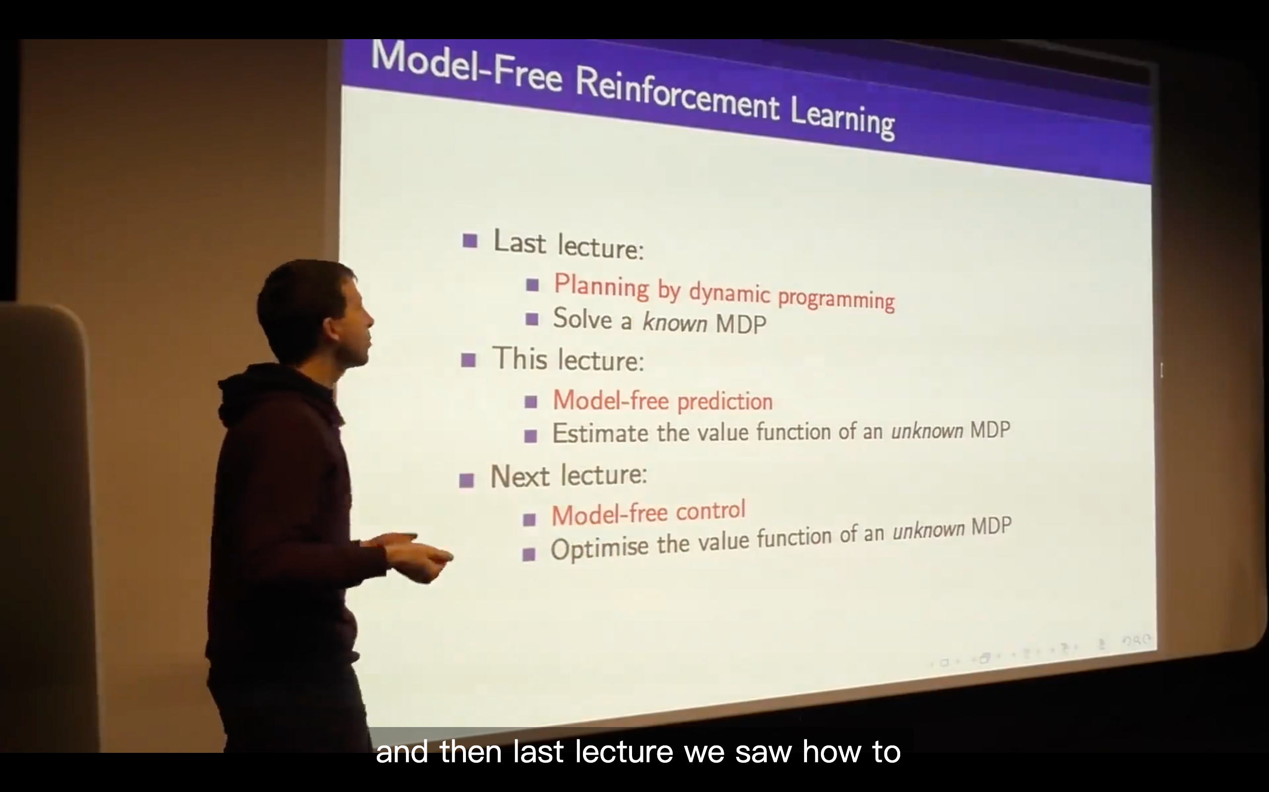
Lecture4: Model-Free Prediction
Introduction
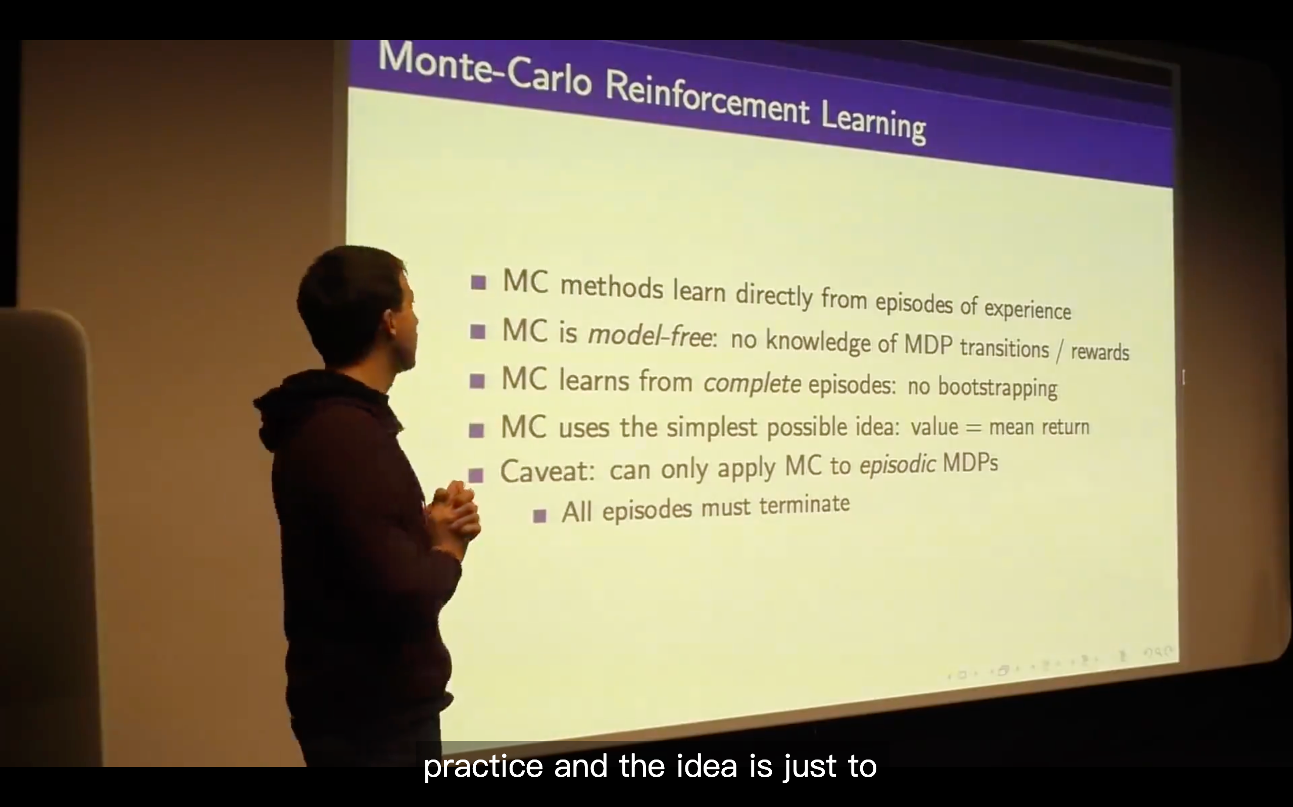
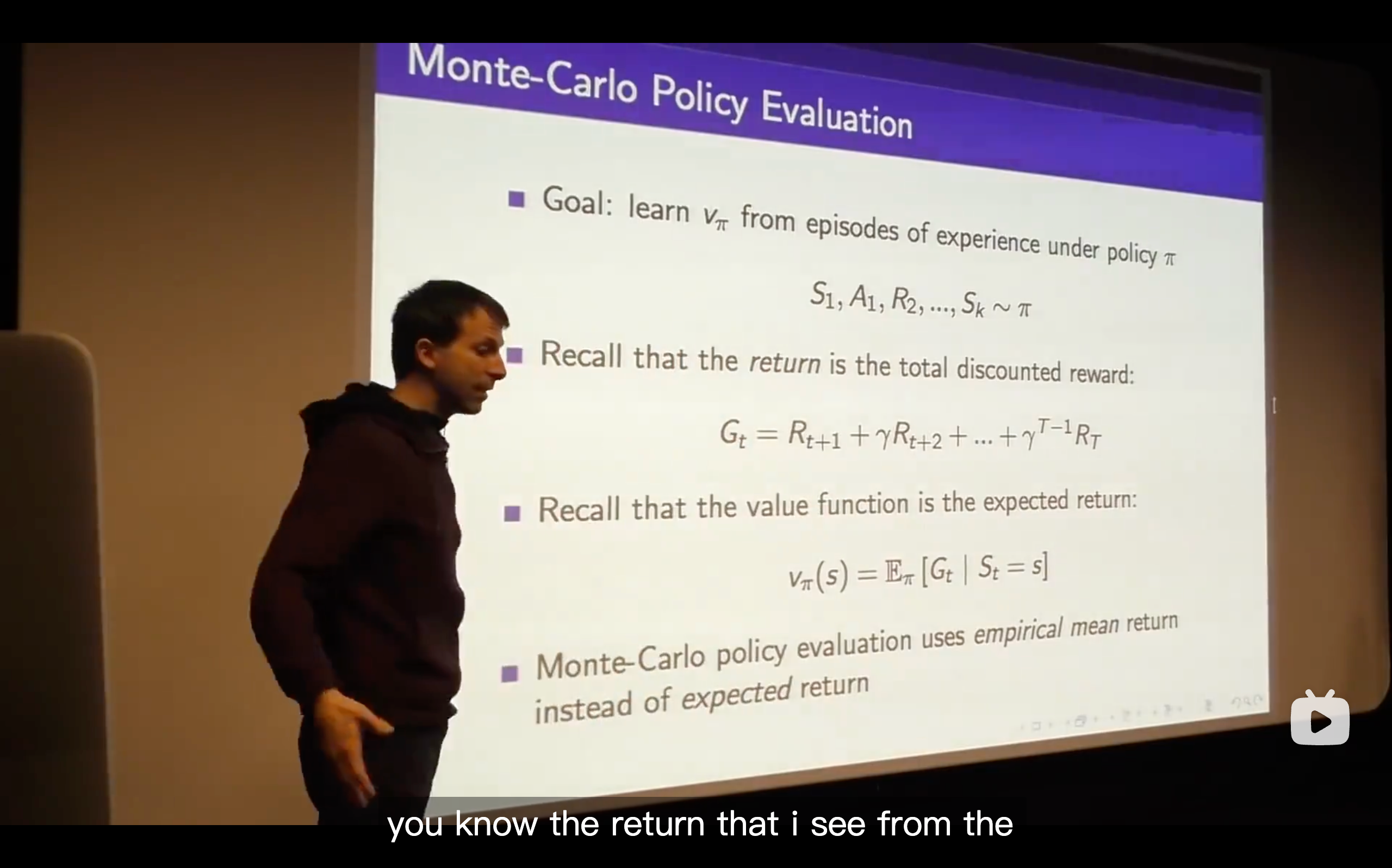
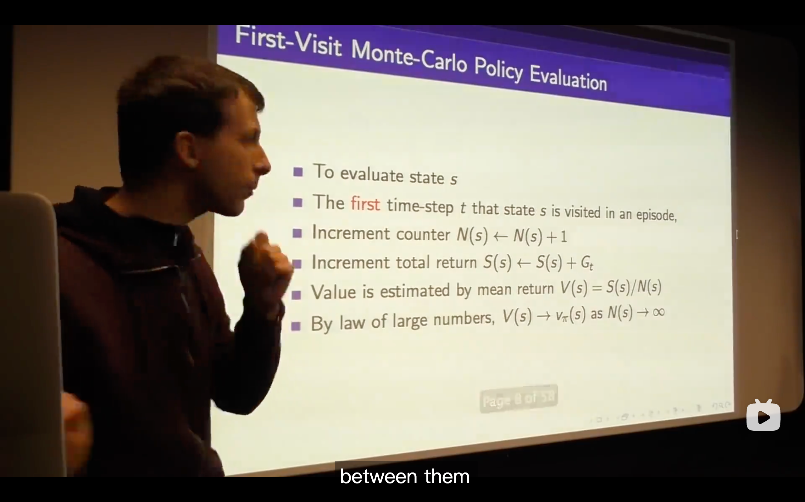
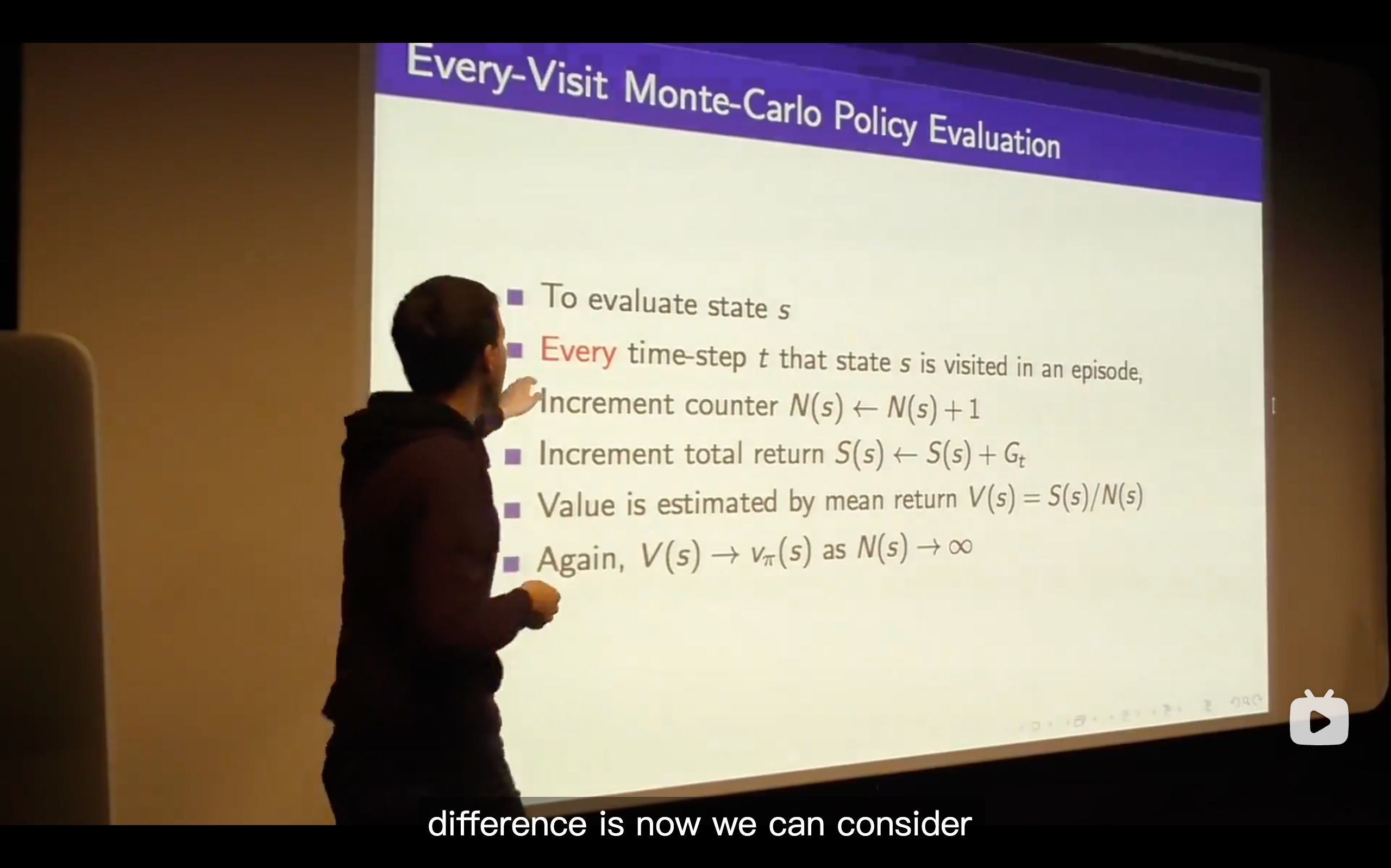
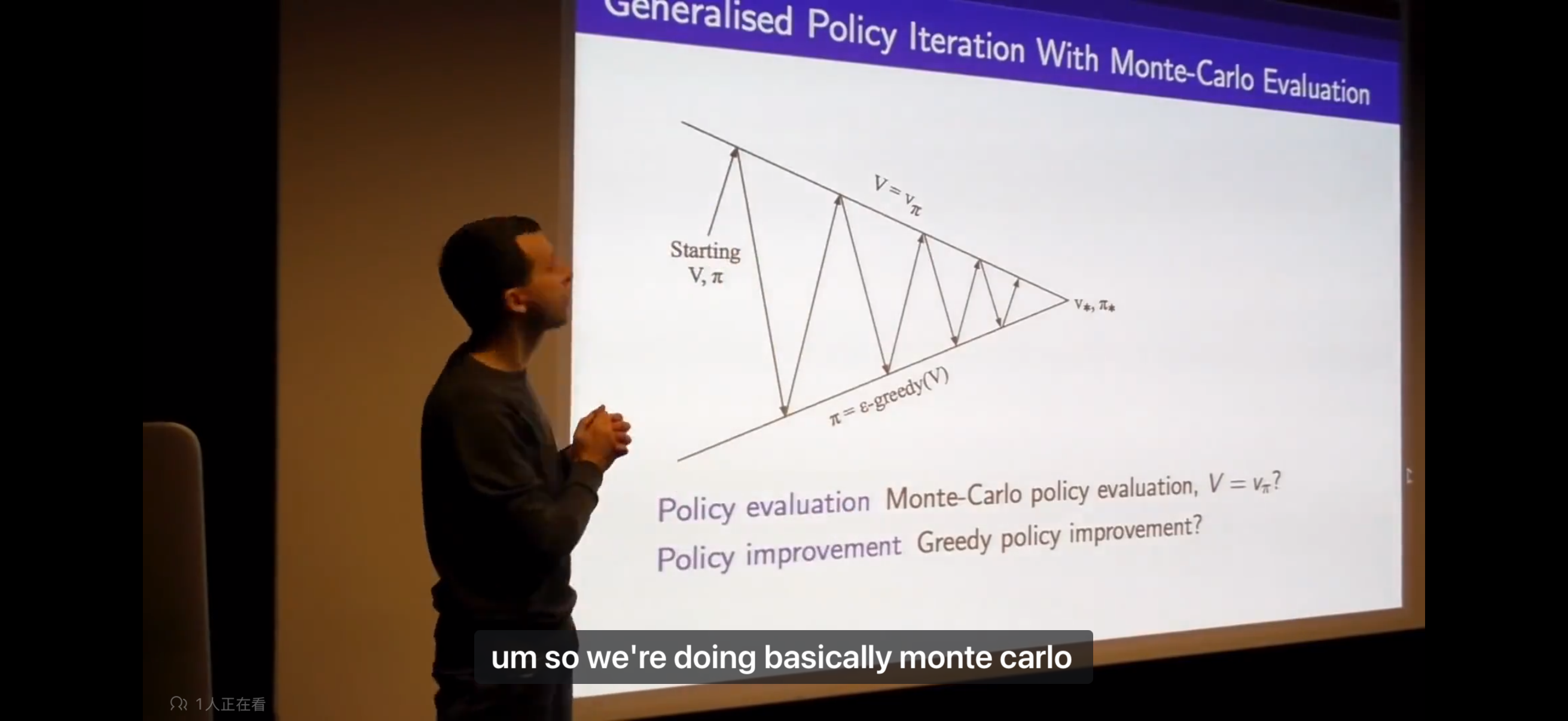
Monte-Carlo Learning
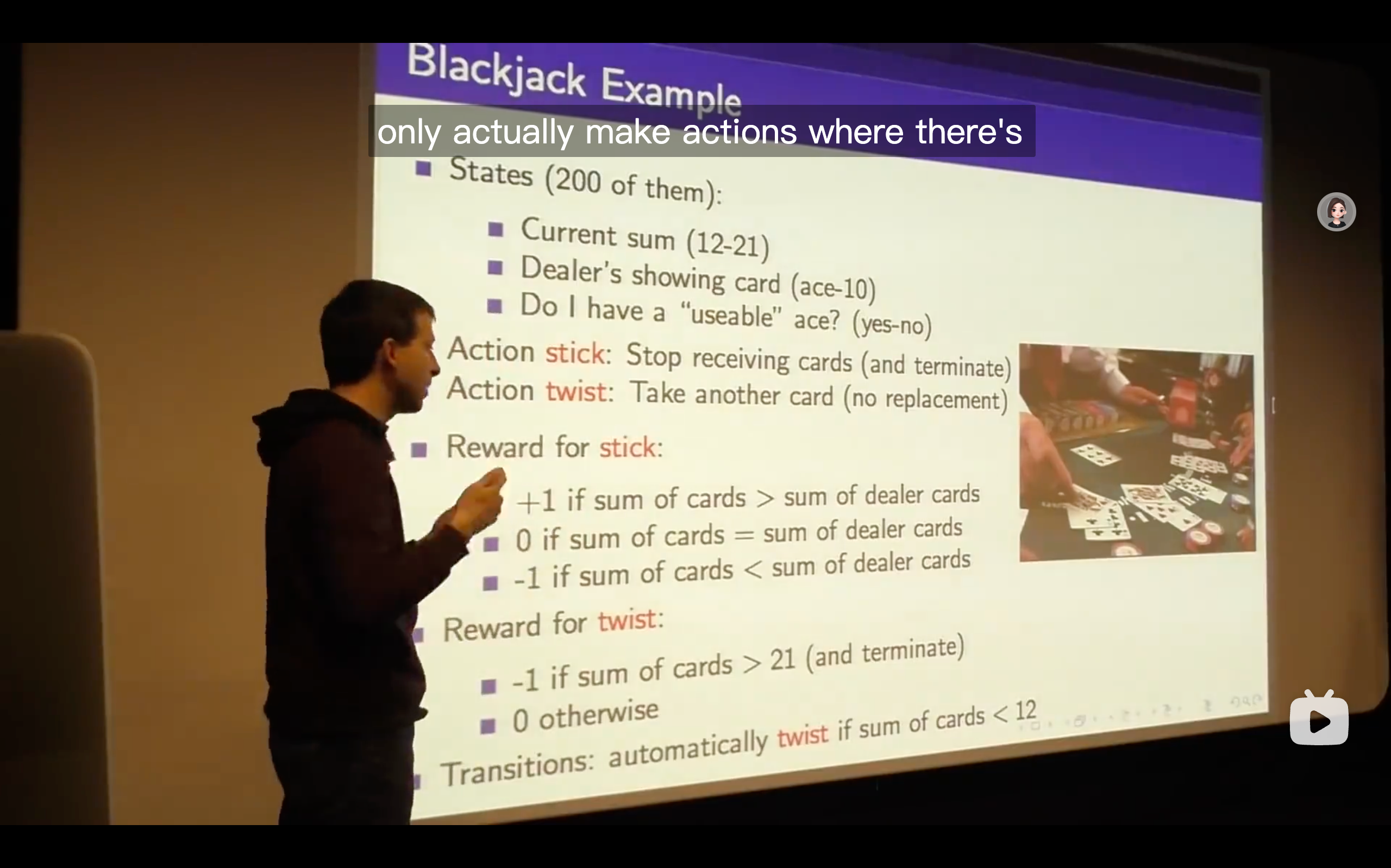
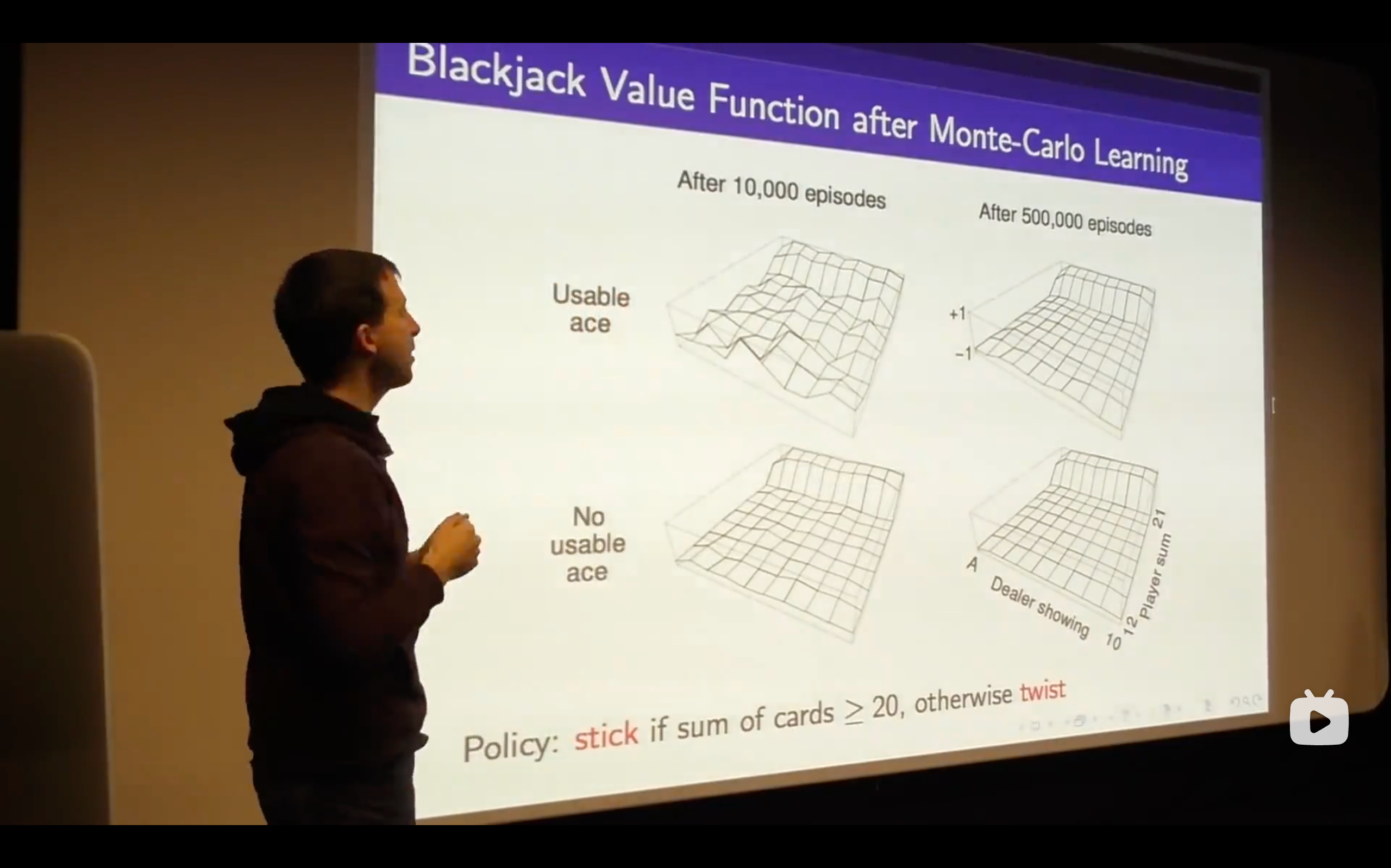
- We see that emerging nicely from the structure of this value function just by sampling, so no one told us the dynamics of the game ( that means no one told us the probabilities that govern yhe game of blackjack), this is just by running episodes, trial and error learning, and figuring out the value function directly from experience.
- The expected reward is the value function.
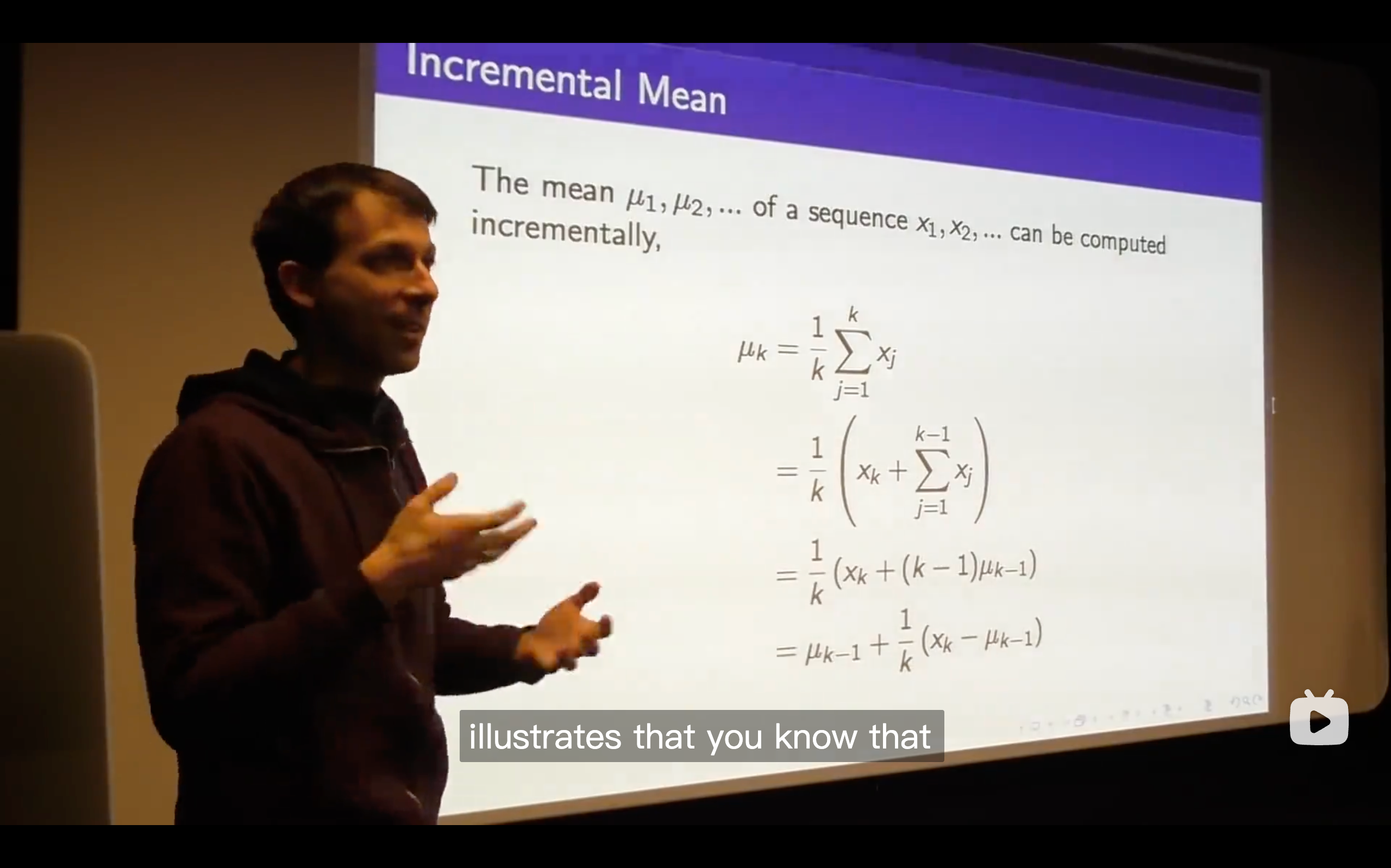
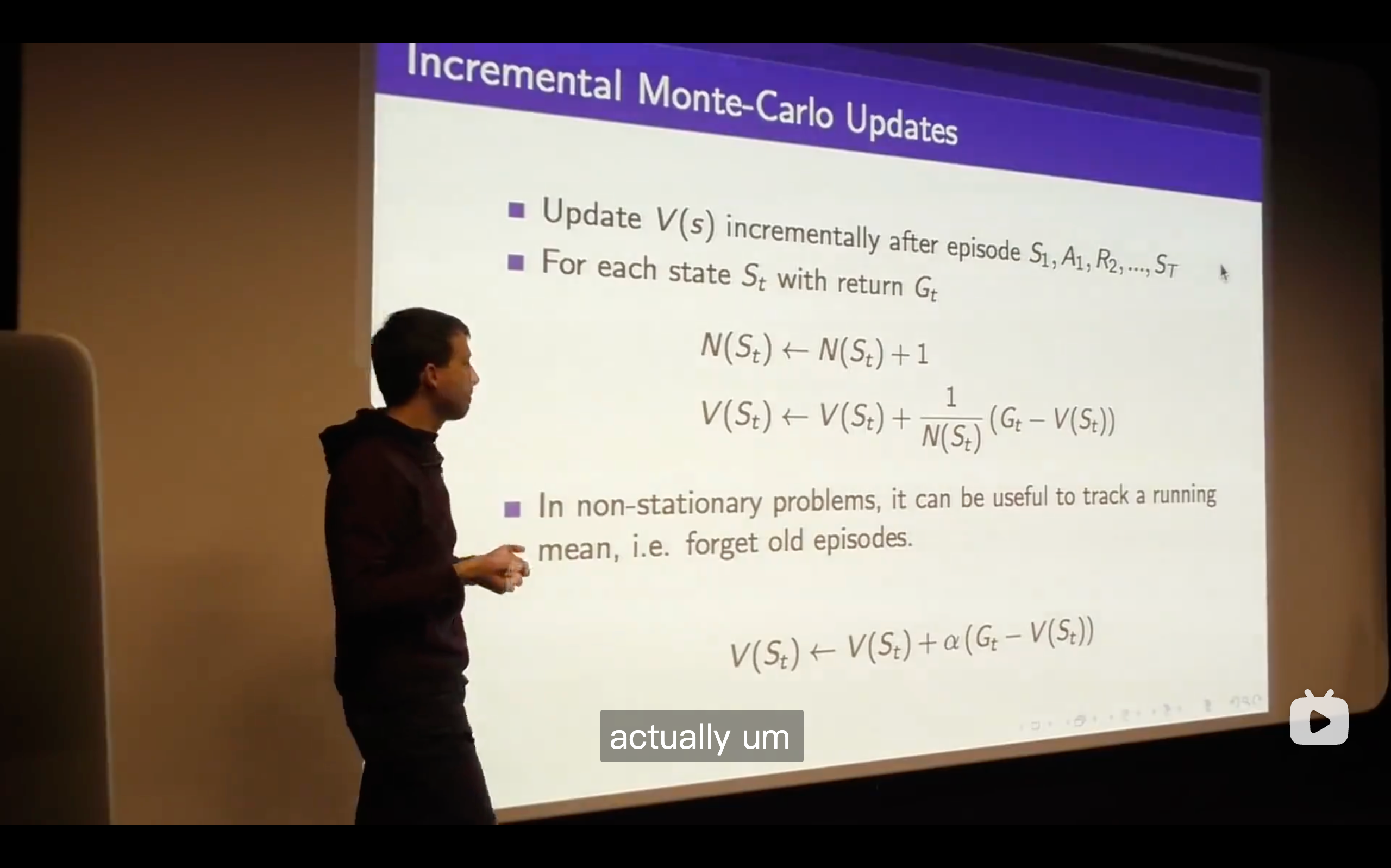
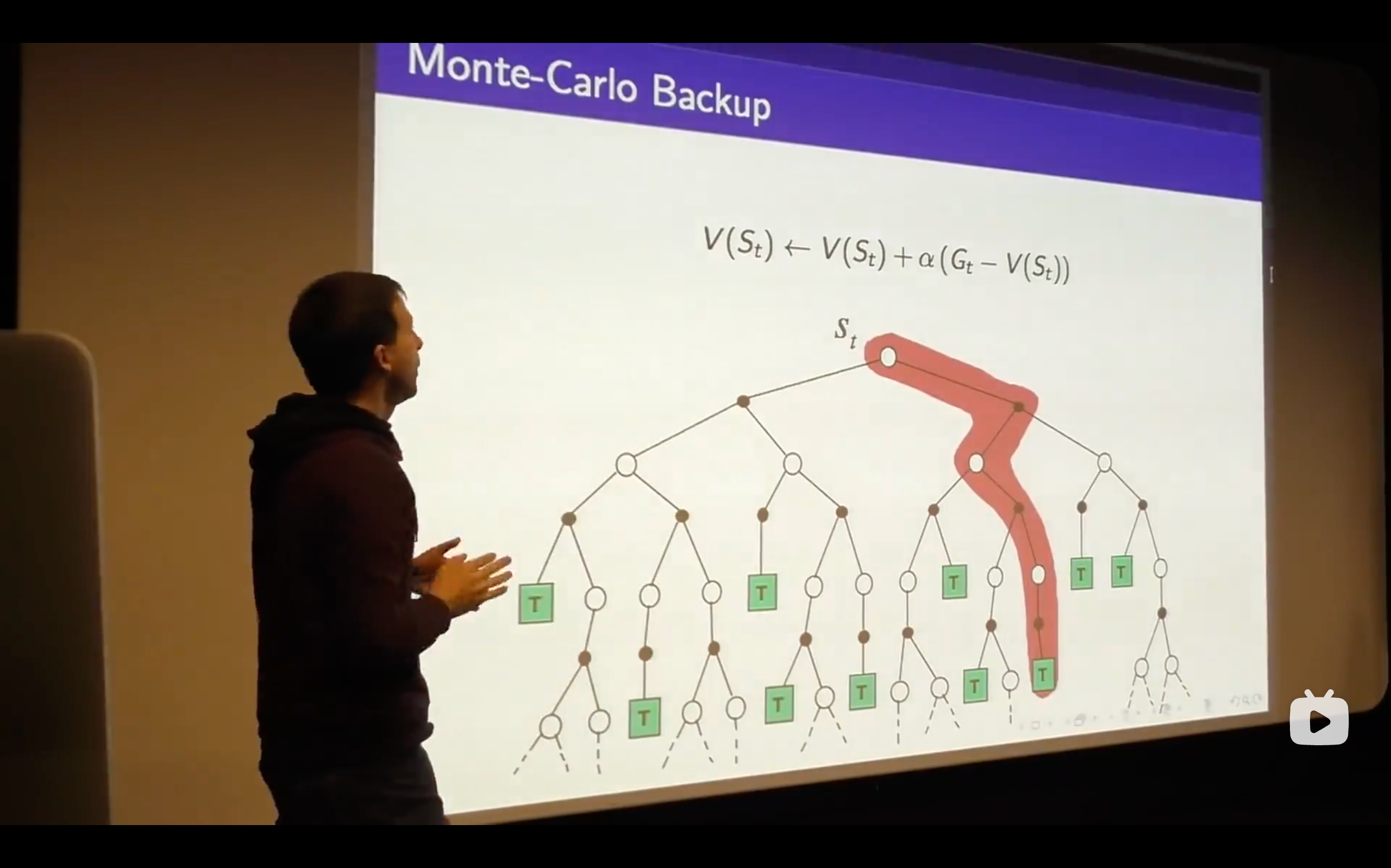
- So that's the Monte-Carlo Learning, a very simple idea that you run out episodes you look at those complete returns that you've seen and you update your estimate of the mean value towards your sample return for each state that you visit.
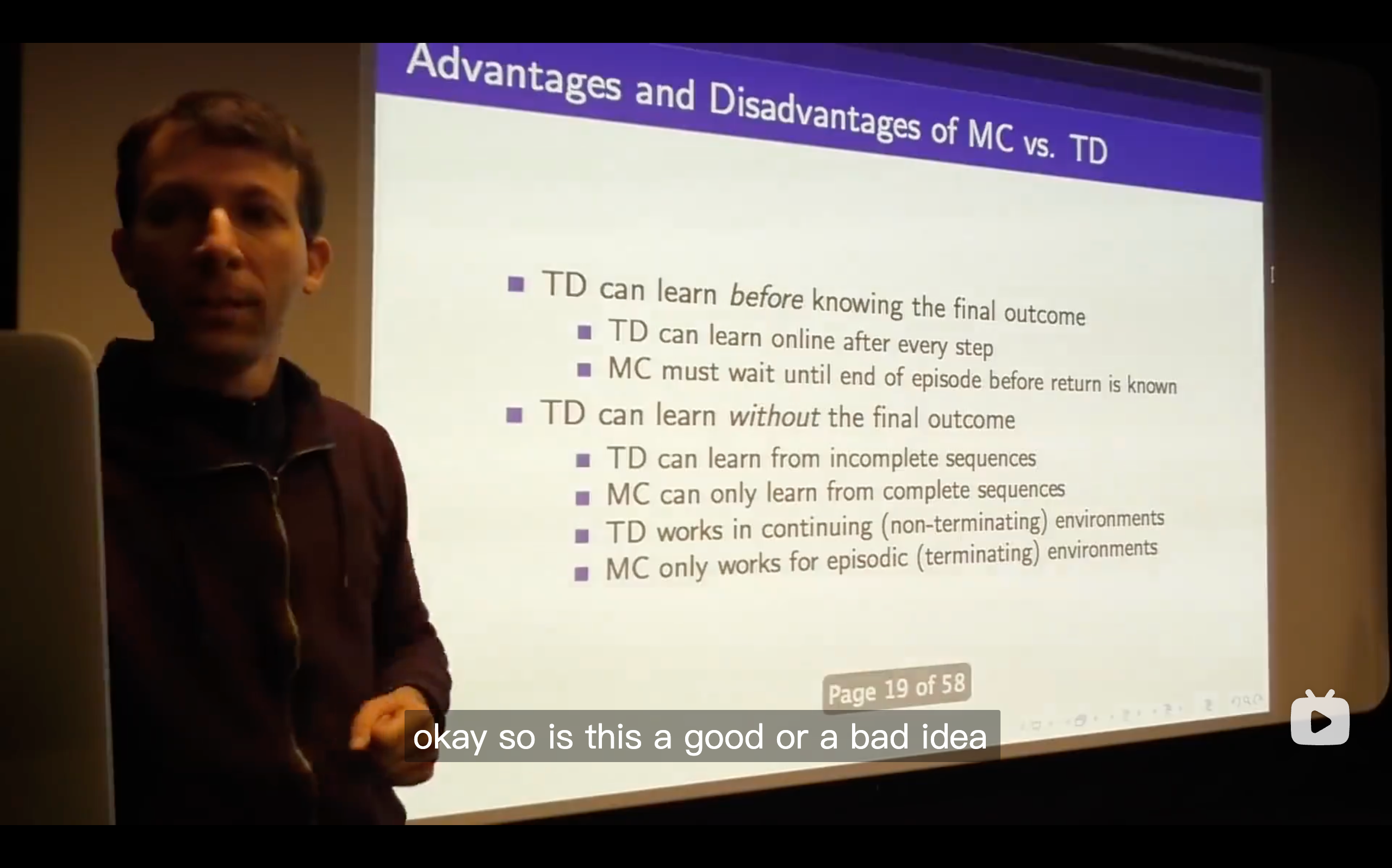
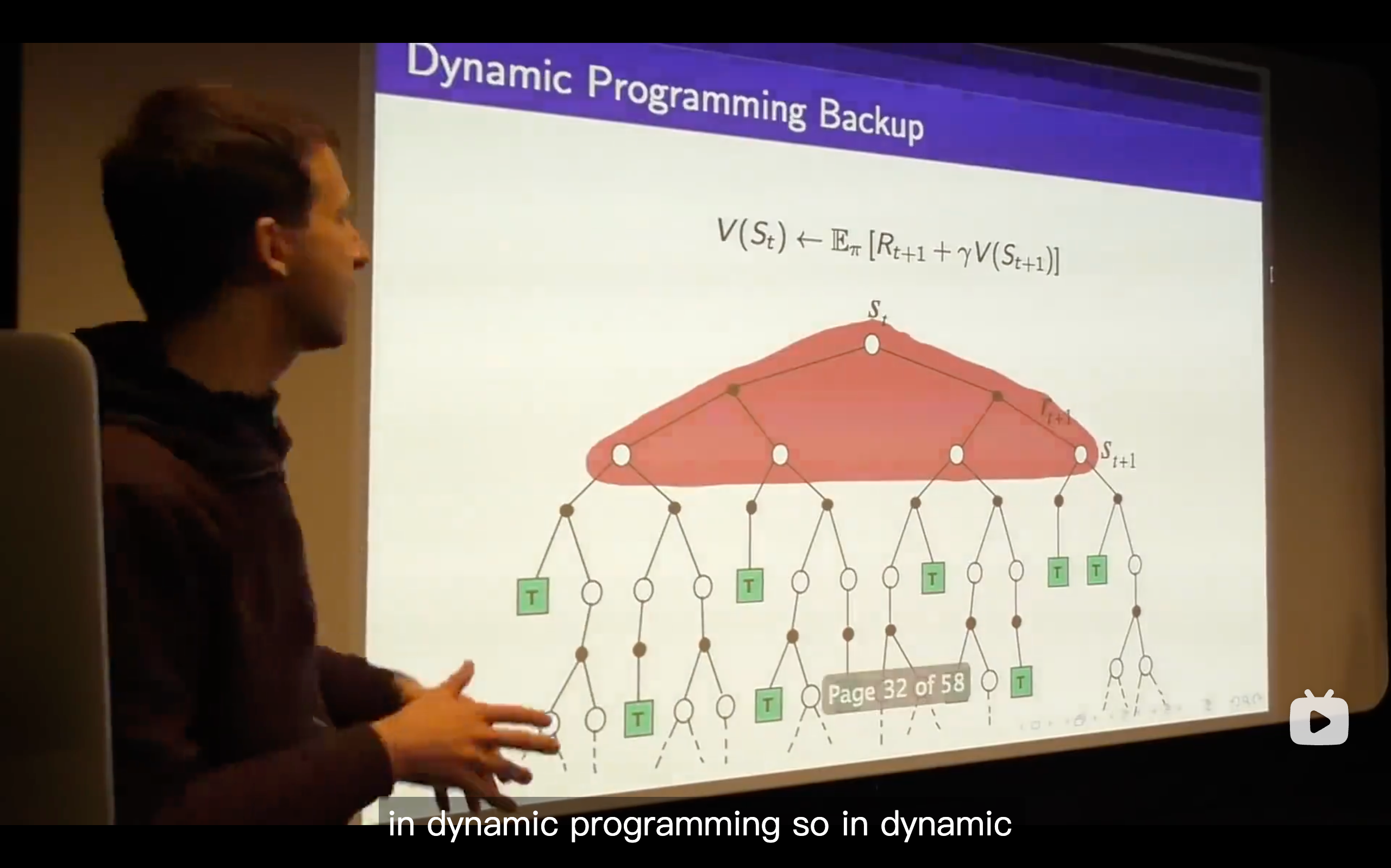
Temporal-Difference Learning
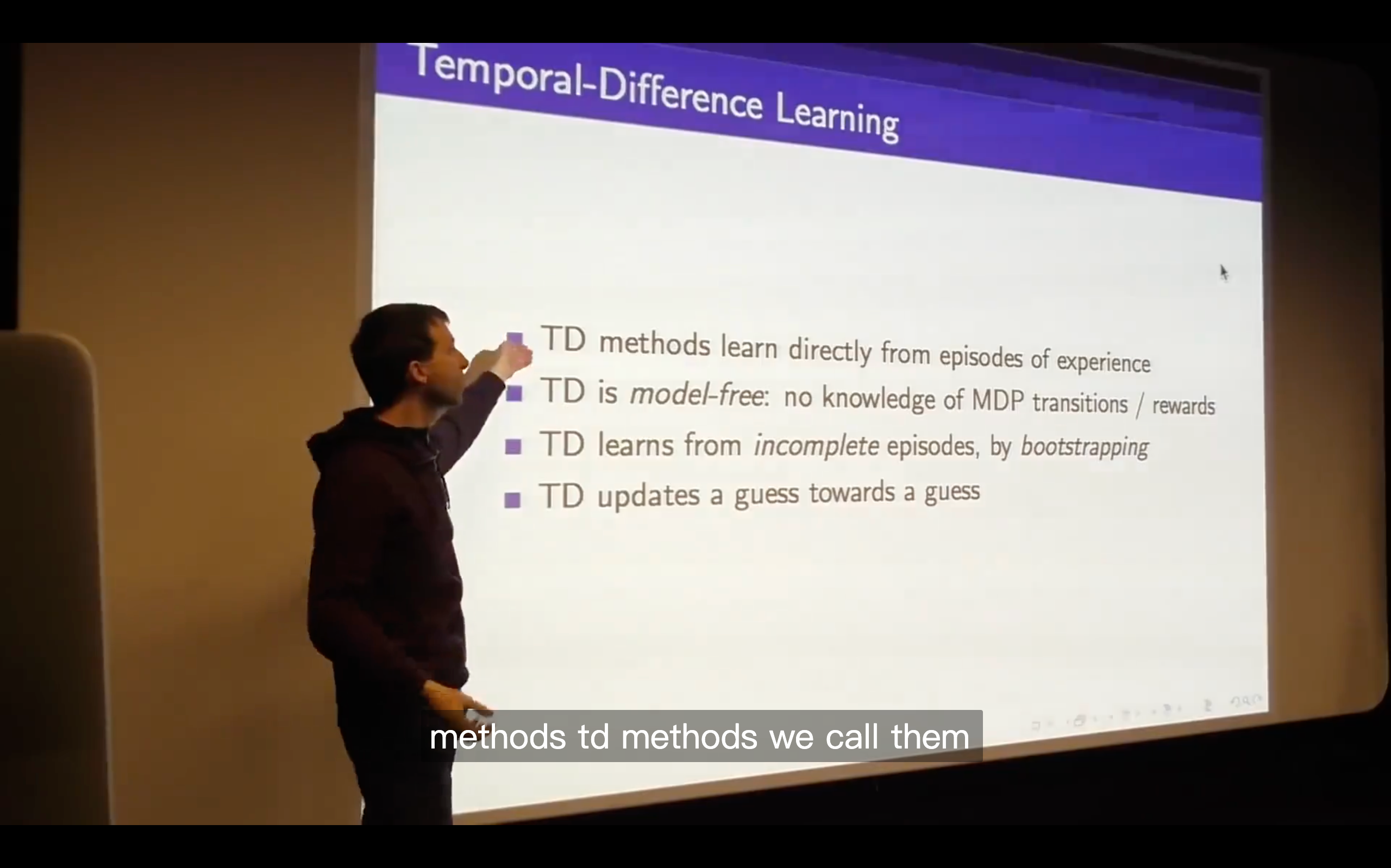
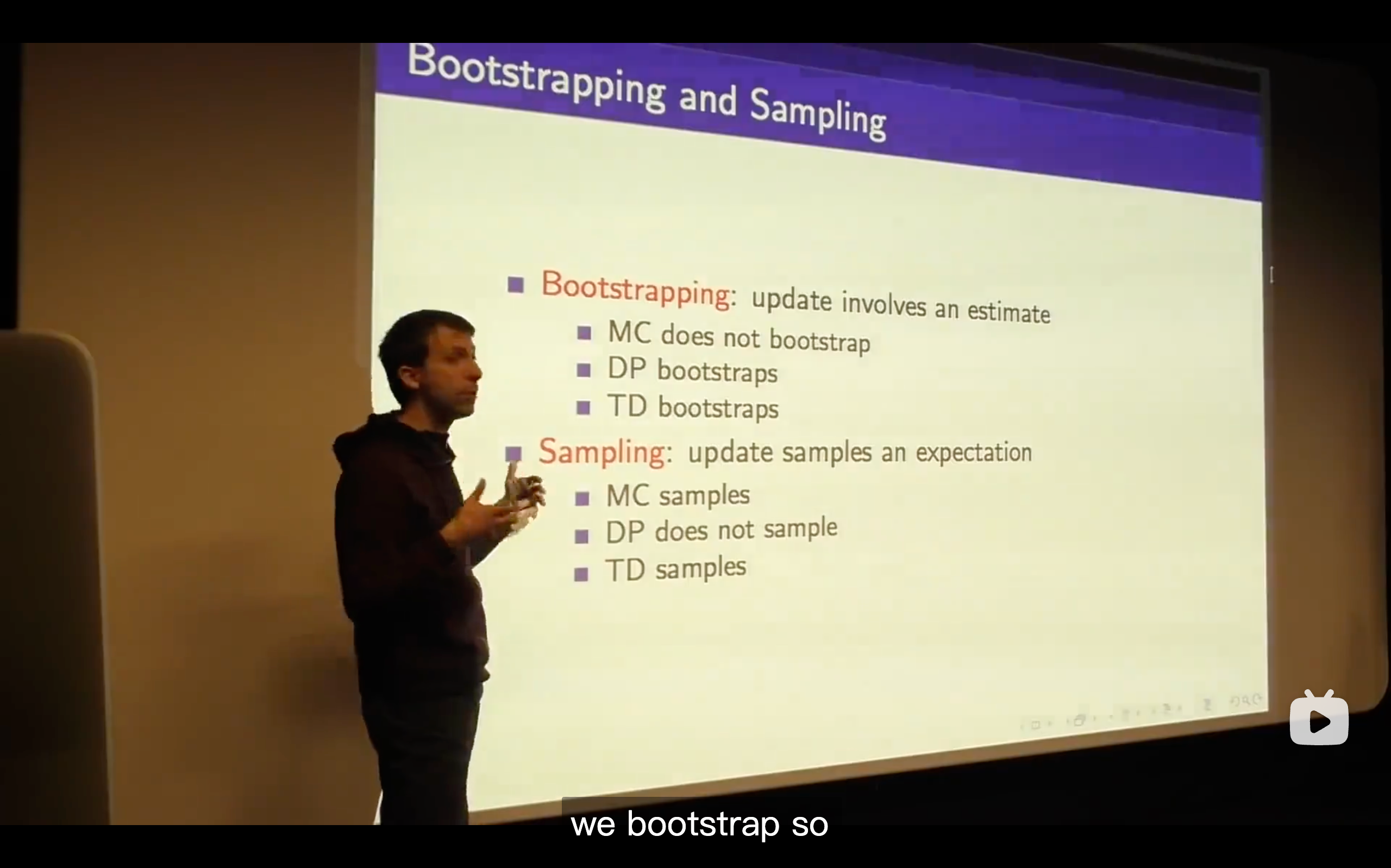
Bootstrapping is the fundamental idea behind TD learning.
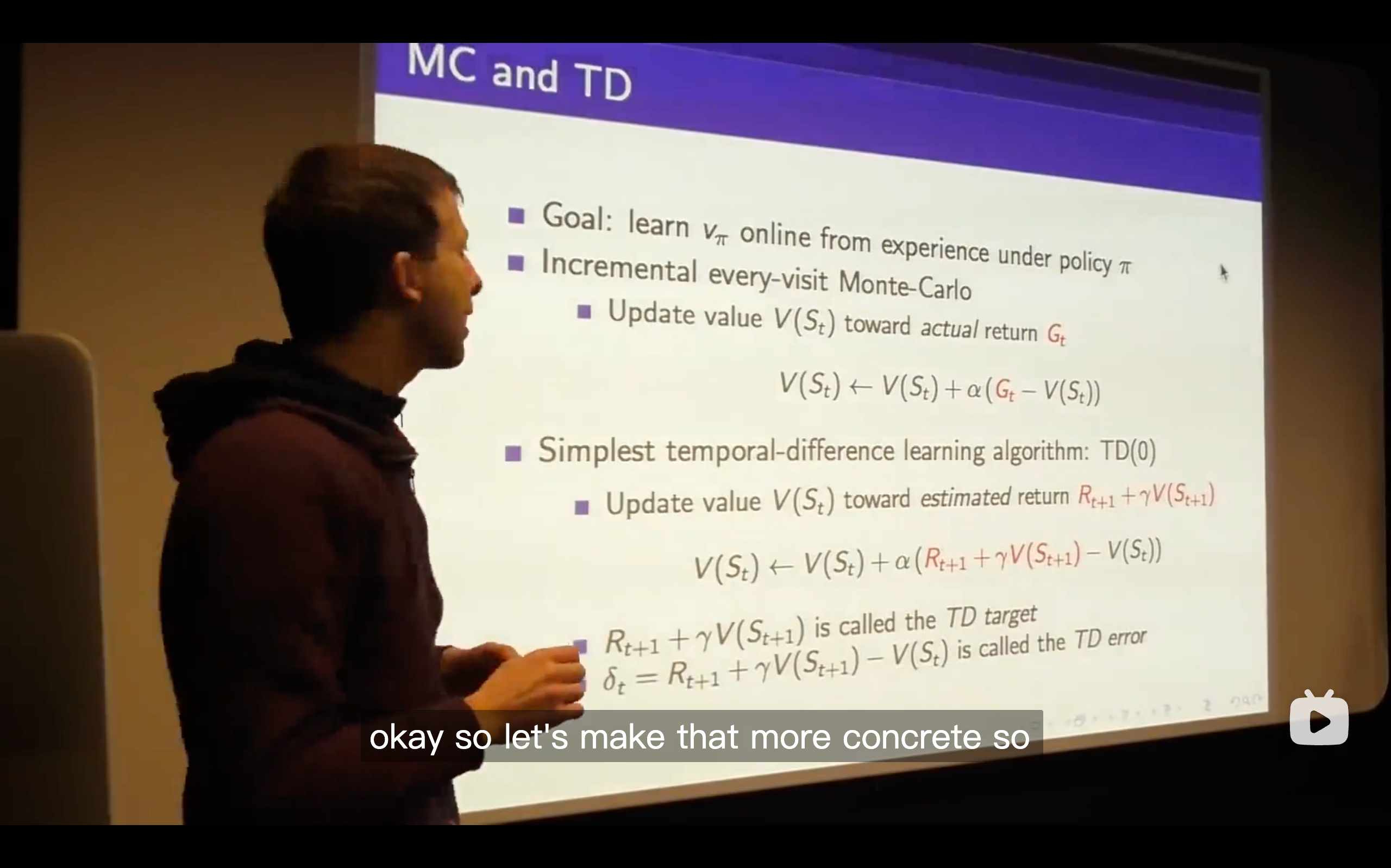
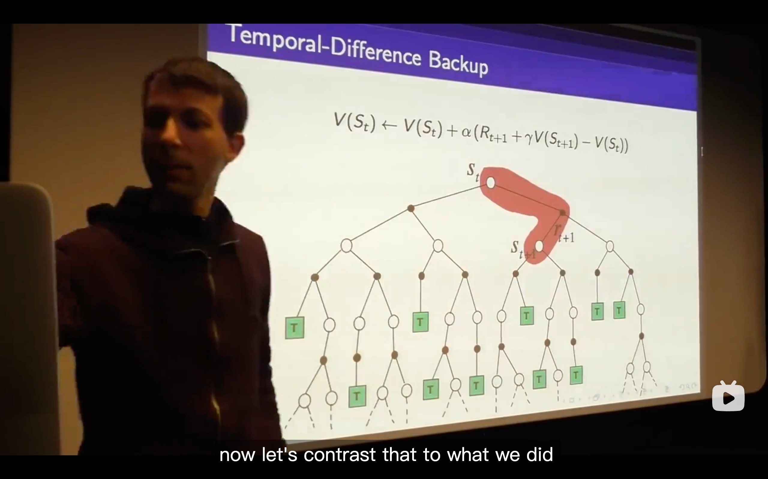
The TD target is like a random target which depends on exactly what happens over the next time step but we get some immediate reward and some value wherever we happen to end up and we're going to move towards that TD target.
In Monte-Carlo, you wouldn't get the negative reward or be able to update your value for your prediction, but in TD learning, you can immediately update the value function you had before and be capable to change your future decision.
We changed our predicted total time based on each state just happened to us.
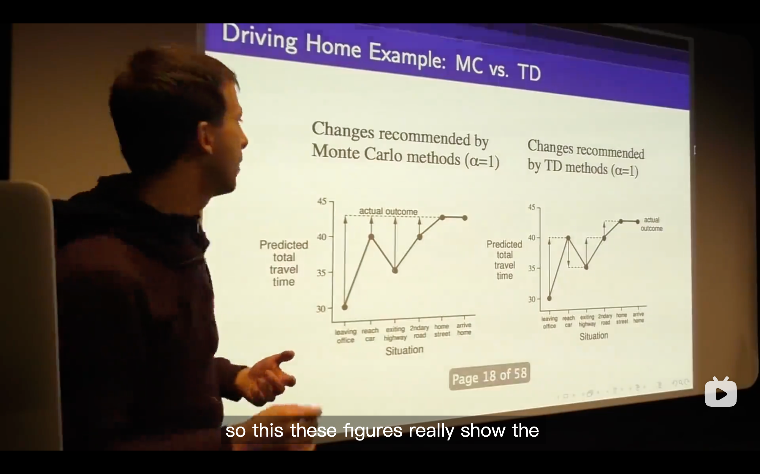
Each step along this when using monte-carlo learning, you update towards the actual outcome you have to wait until you finally get the final state, seeing the actual travel time and then updating each of your value estimates along the way.
.Whereas with TD learning it's quite different. At every step, it's like you started off thinking it's going to take you how long, after one step you thought can be changed. So in other words, you can immediately update your predicted total travel time instead of waiting until anything else happened.
What's the meaning of TD learning?
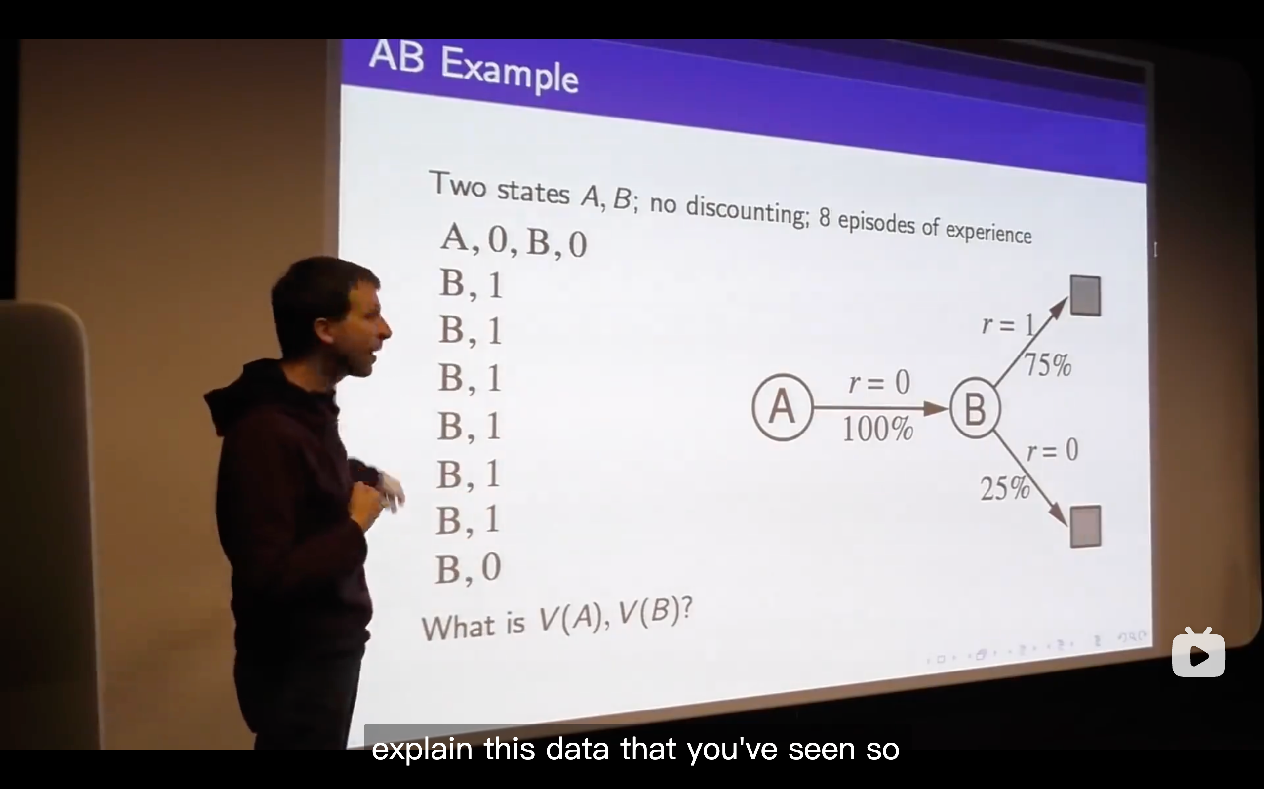
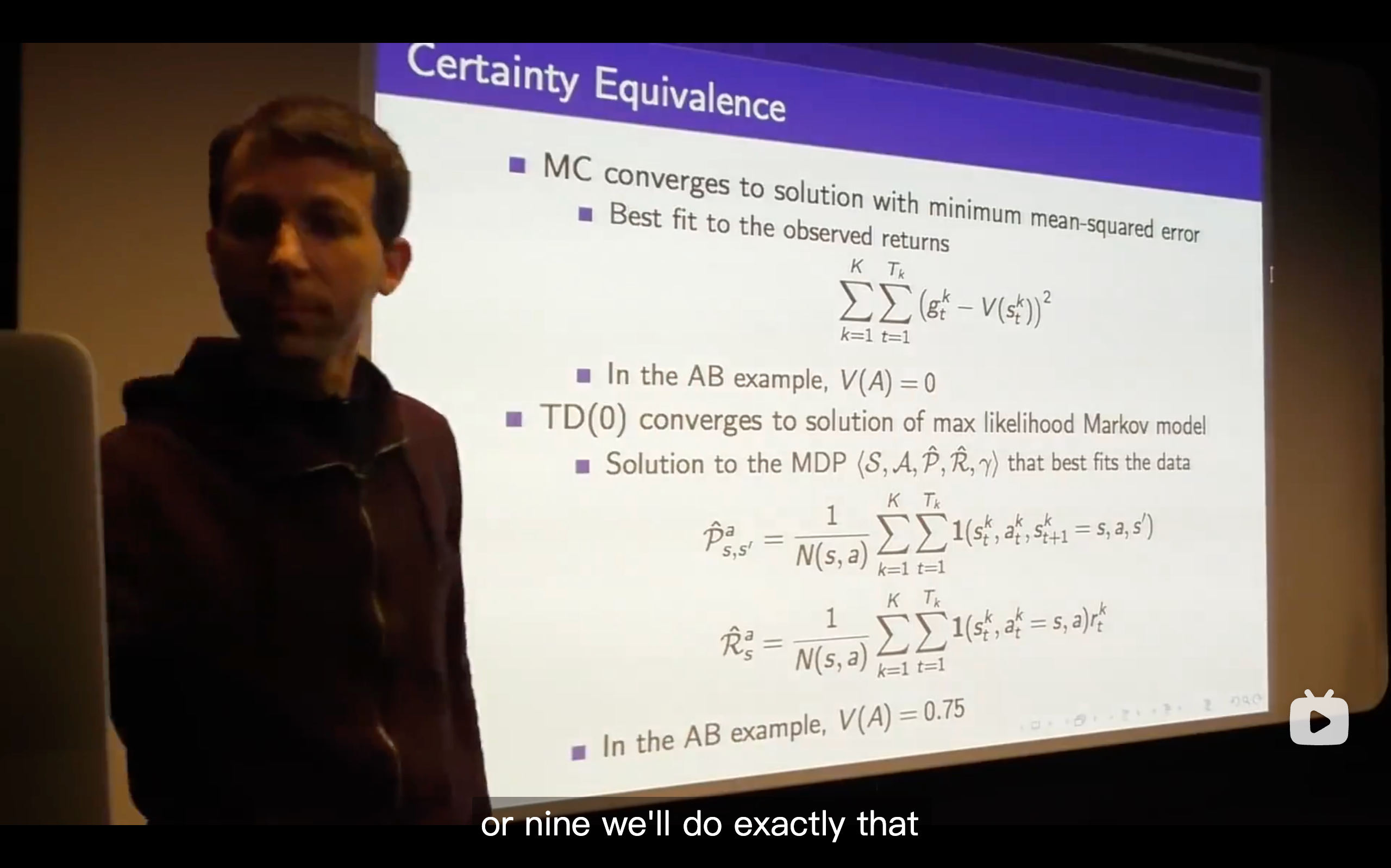
- The basic answer is that in the TD, it finds the true value function as long as you run this thing out, it will always ground itself because even though you correct yourself based on your guess and that guess might not be right, that guess will then be updated towards something that happens subsequently which will ground it more and more, so all of your guesses are progressively becoming better and that information backs up such that you get the correct value function.
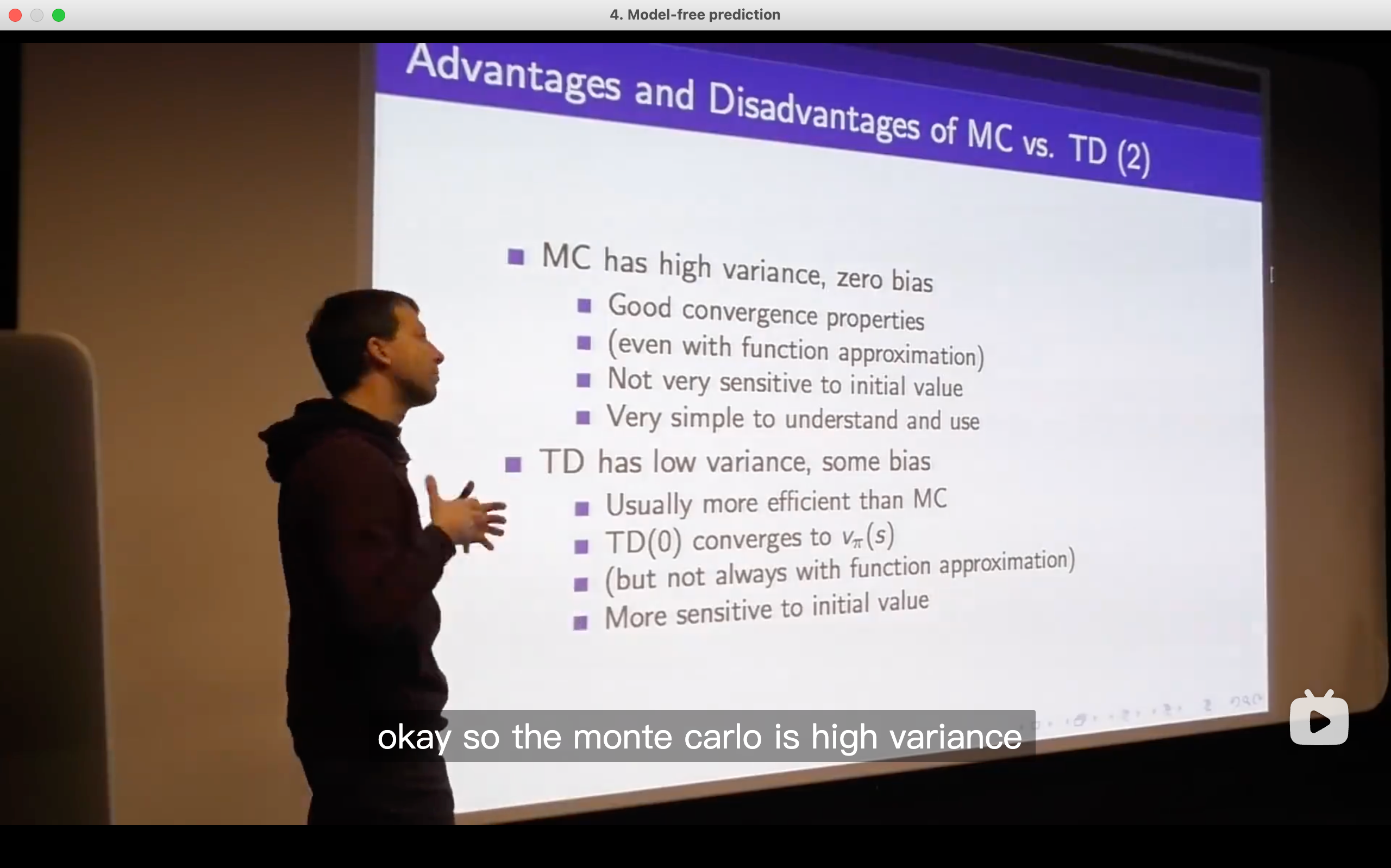
- TD is trying to explain the data in the best possible way.
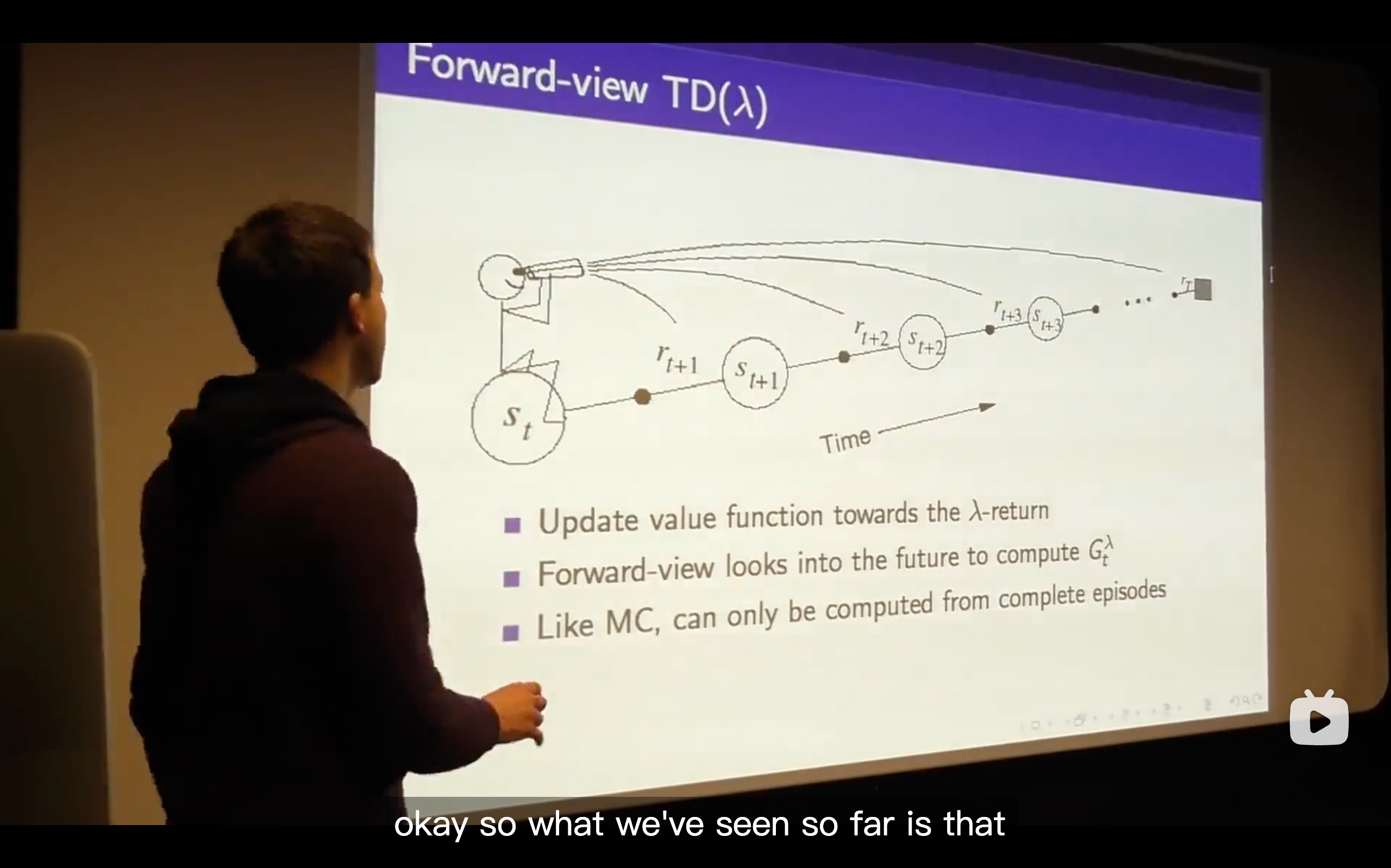
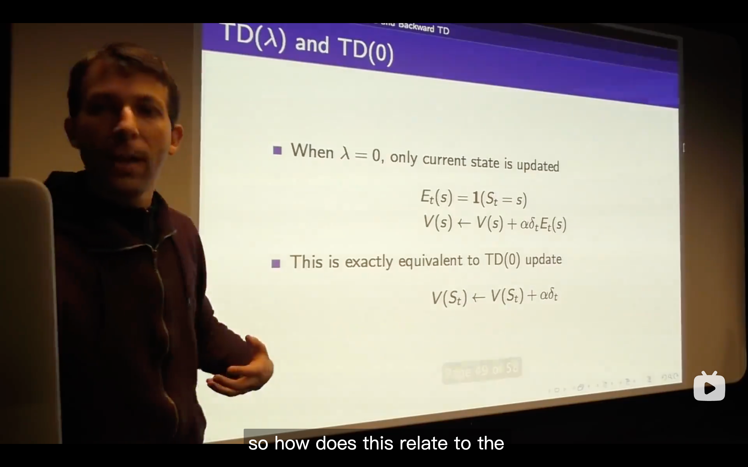
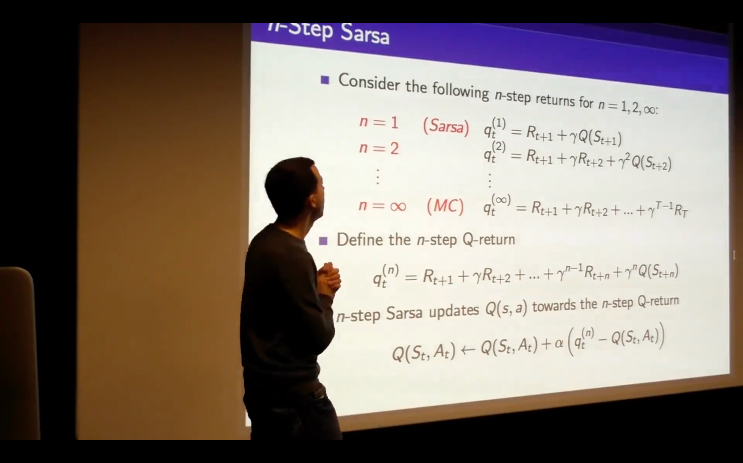
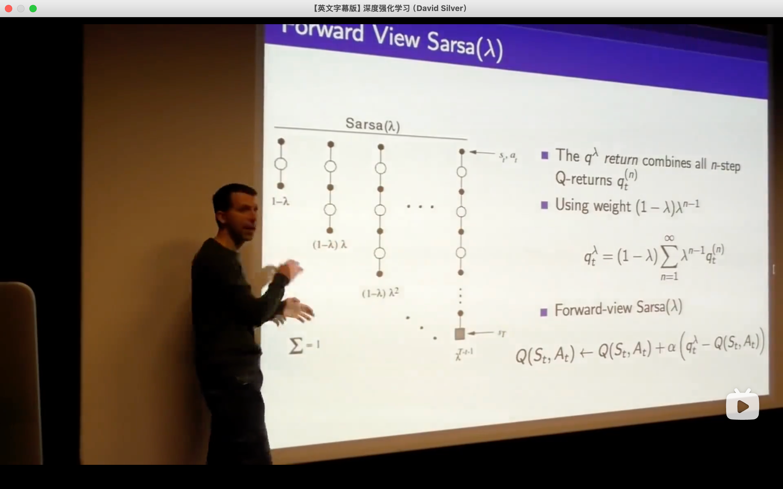
TD(
) (The generlizing function of TD learning, which enhancing the n from 1 to endless.) 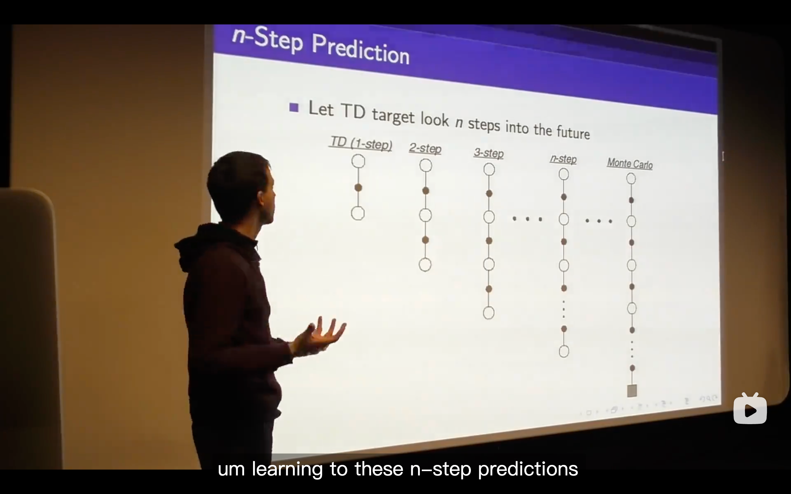
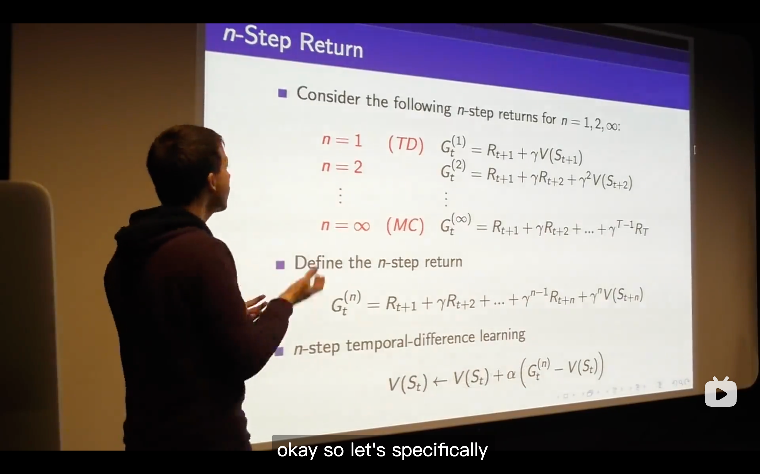
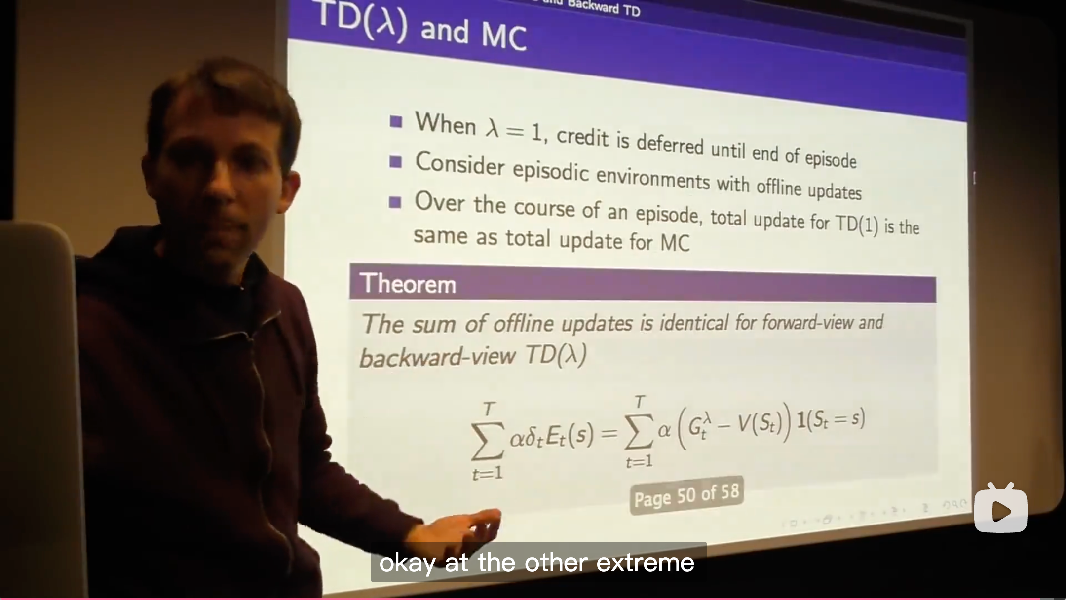
- What we talk about is just whether we do online or off-line updates and that means whether we immediately update our value function or whether we defer the updates of our value function until the end of the episode.
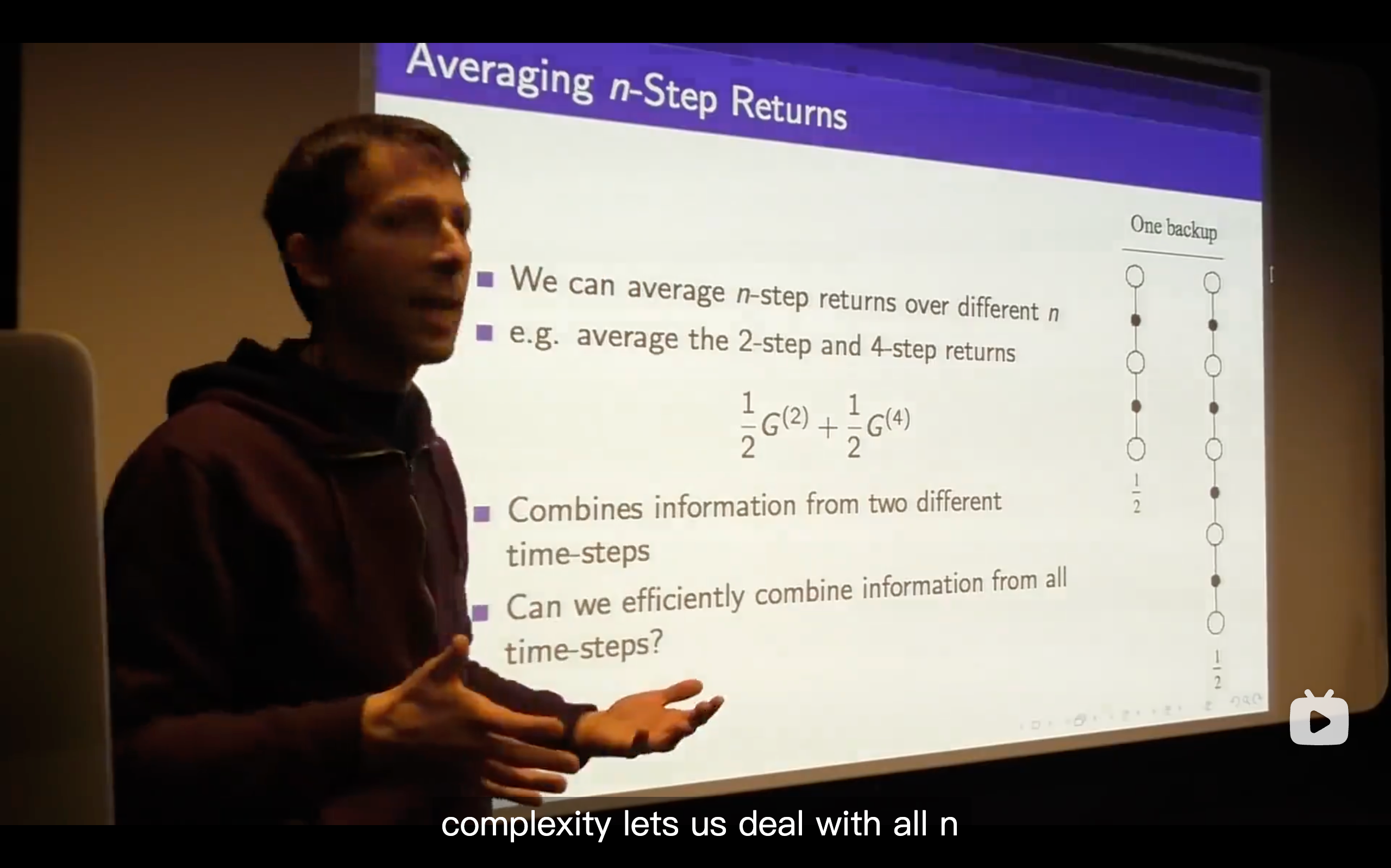
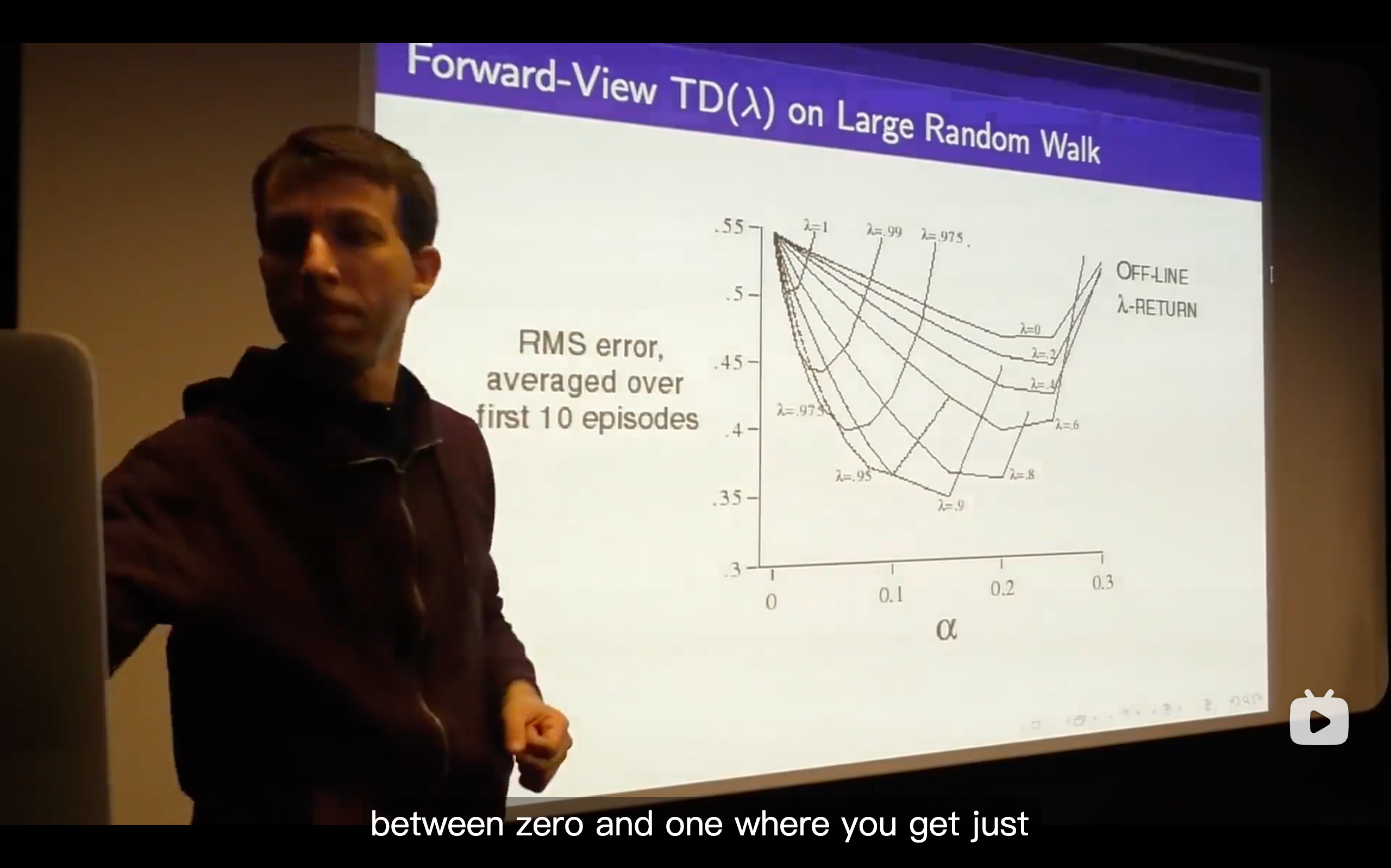
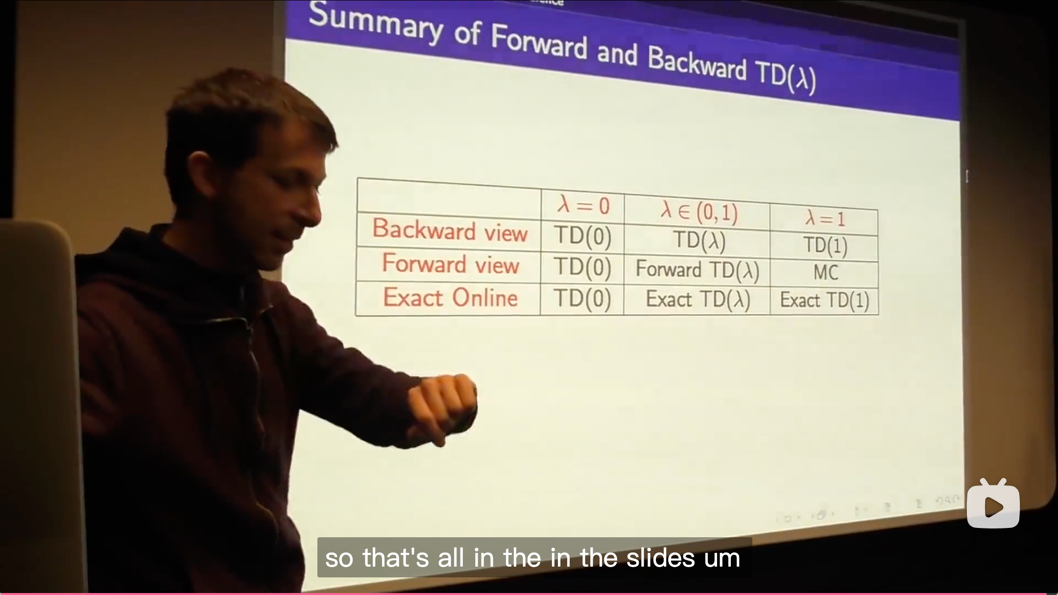
- So what we're going to do is trying to come up with the best all of n and that's the goal to efficiently consider all n at once.
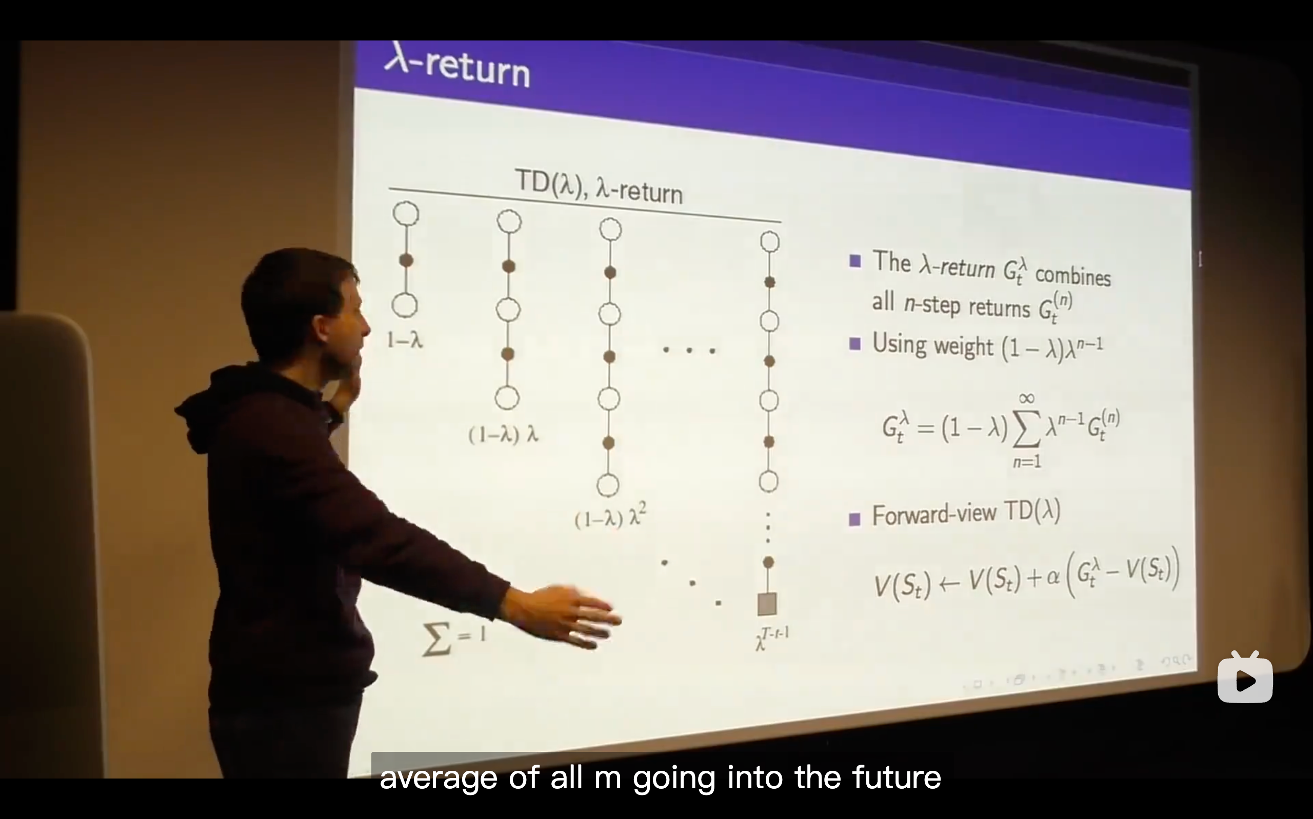
- (1 -
) is a normalizing factor. 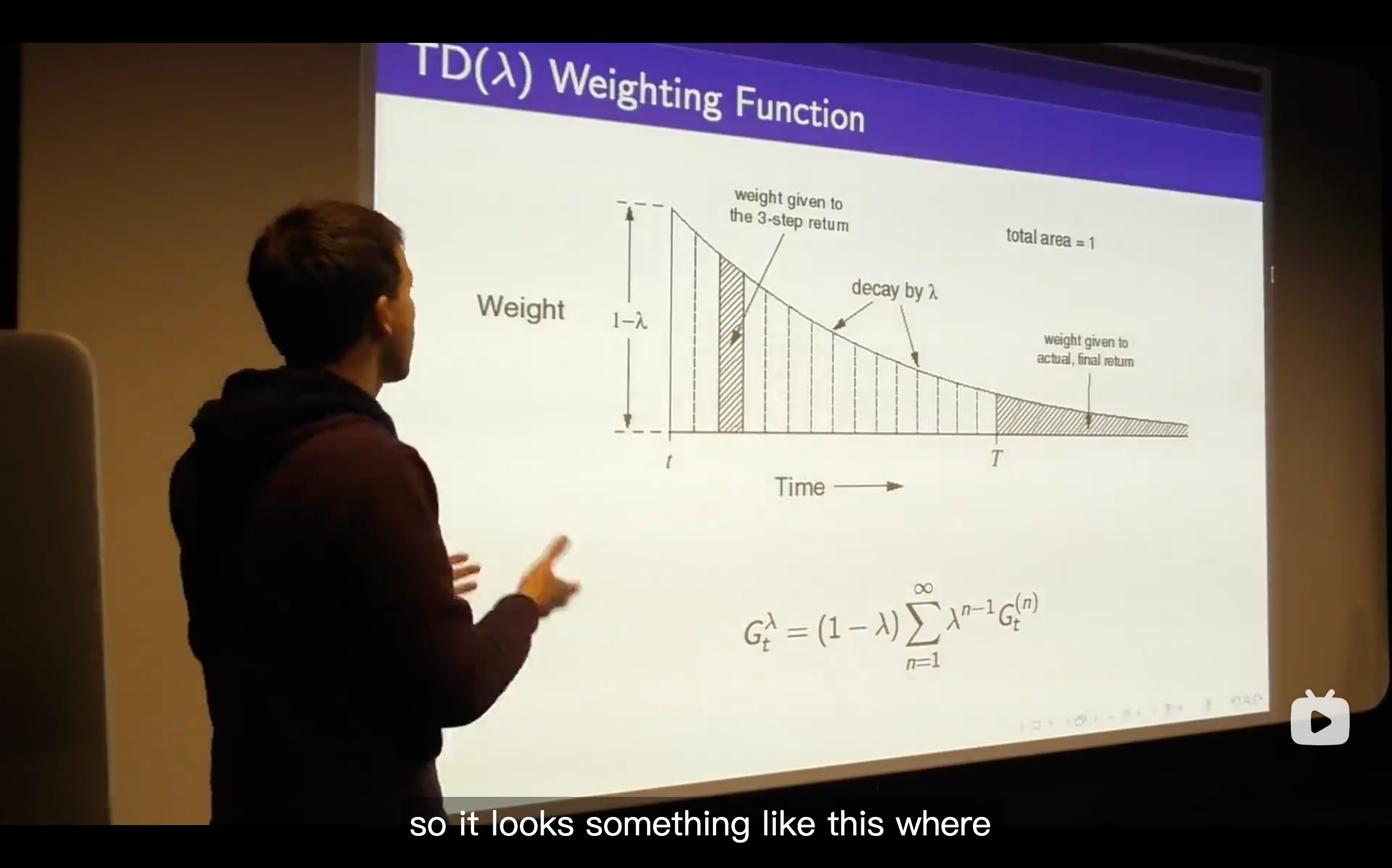
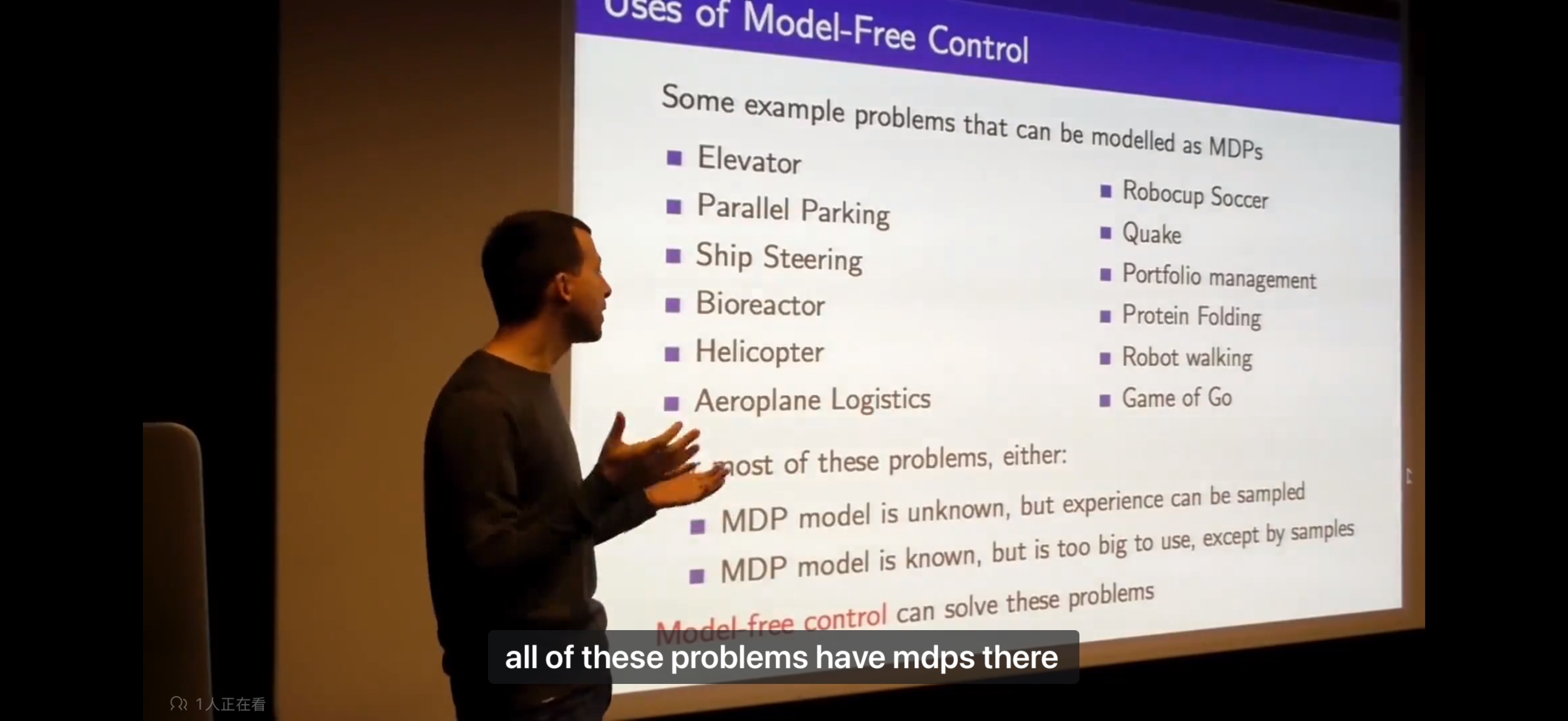
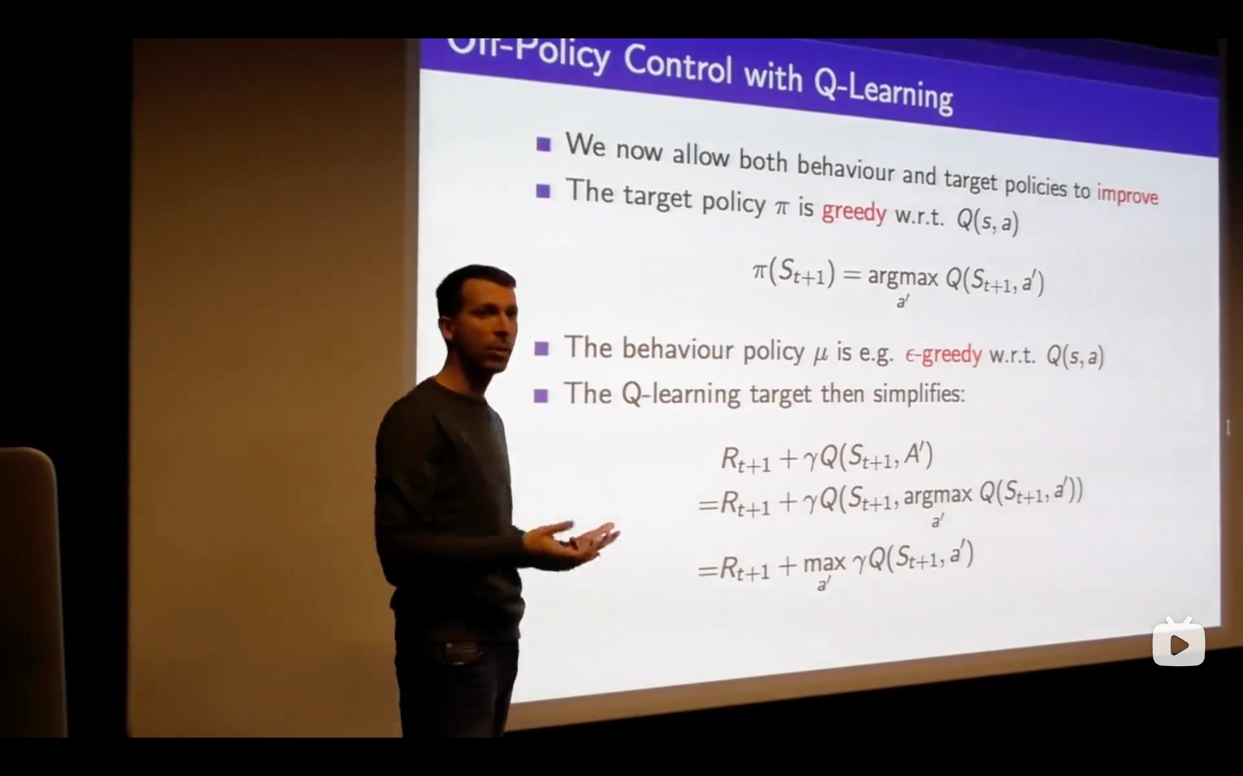
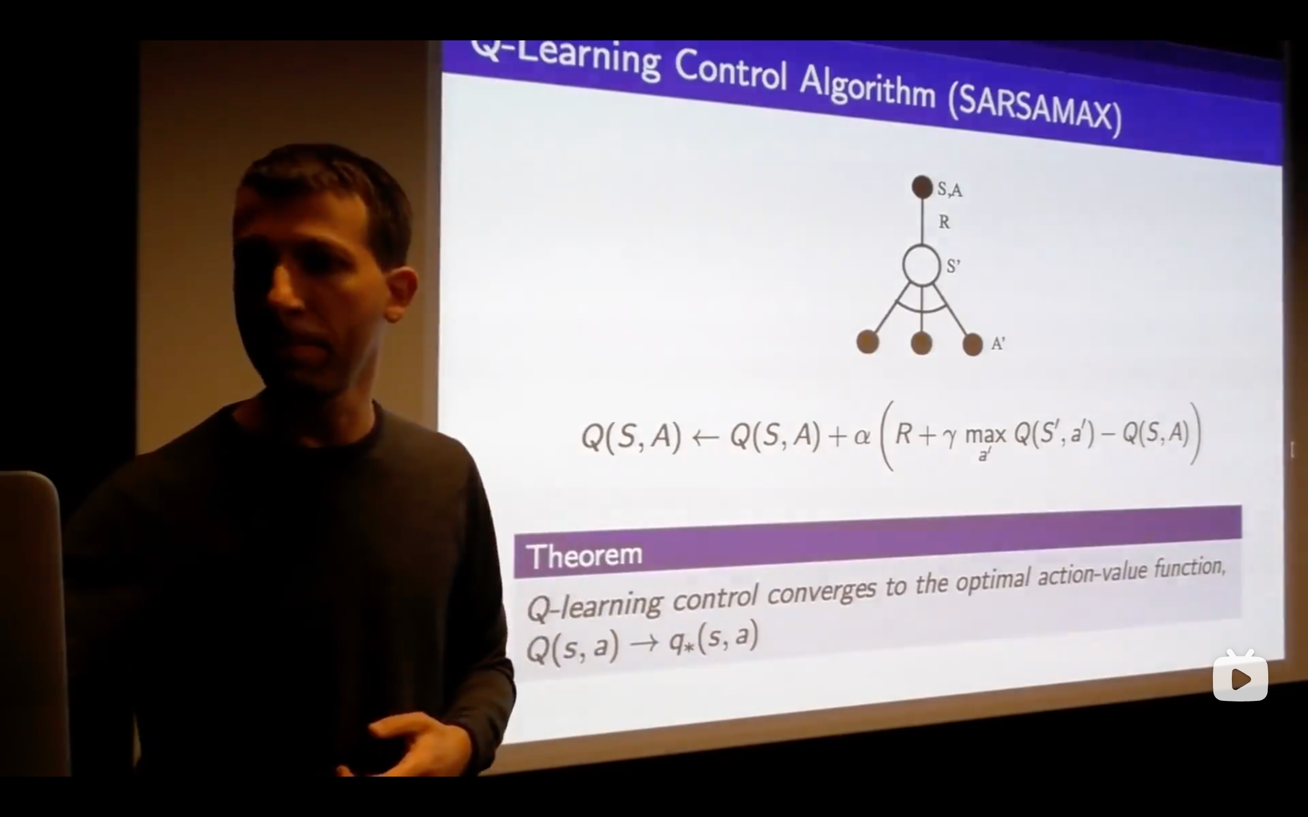
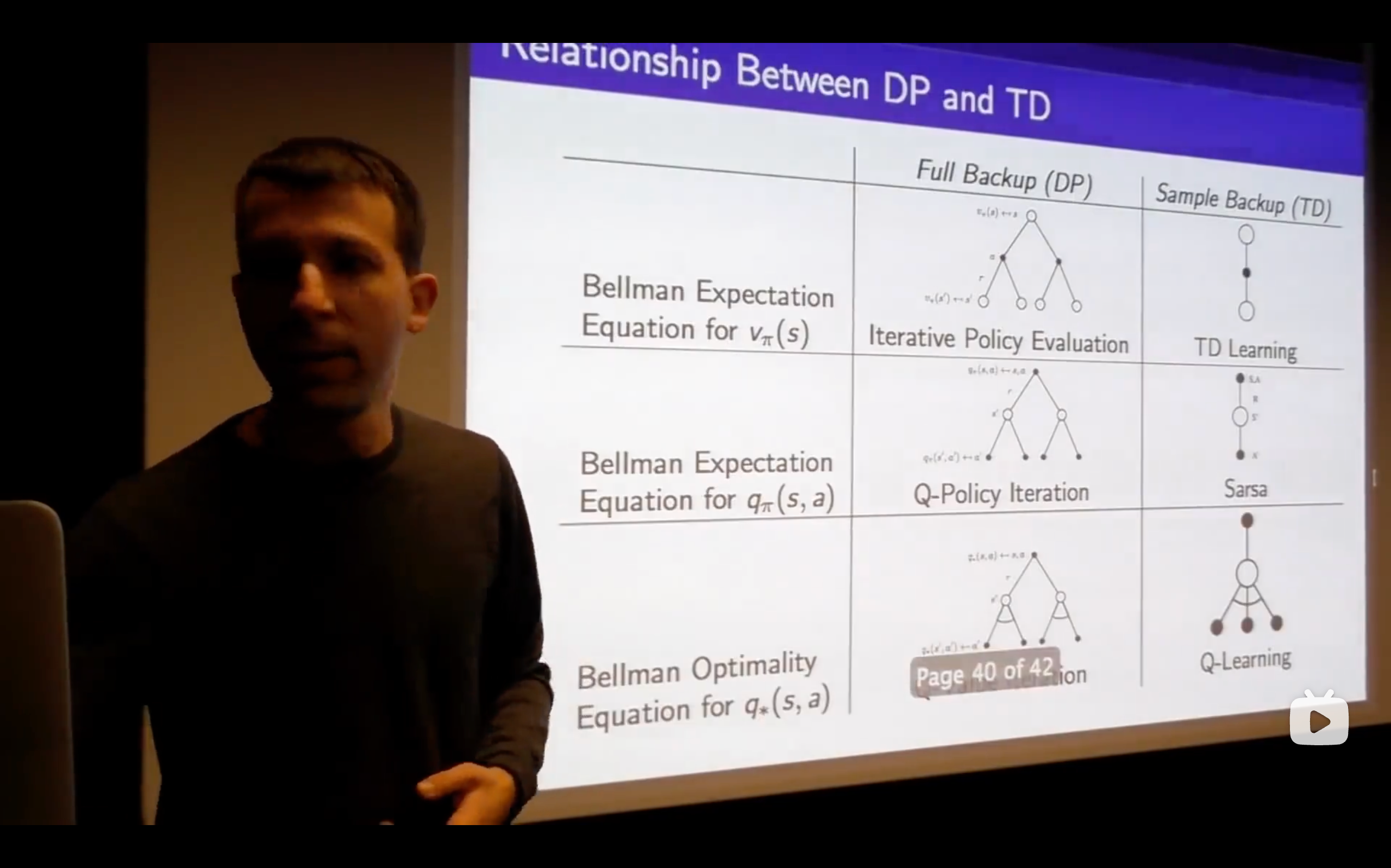
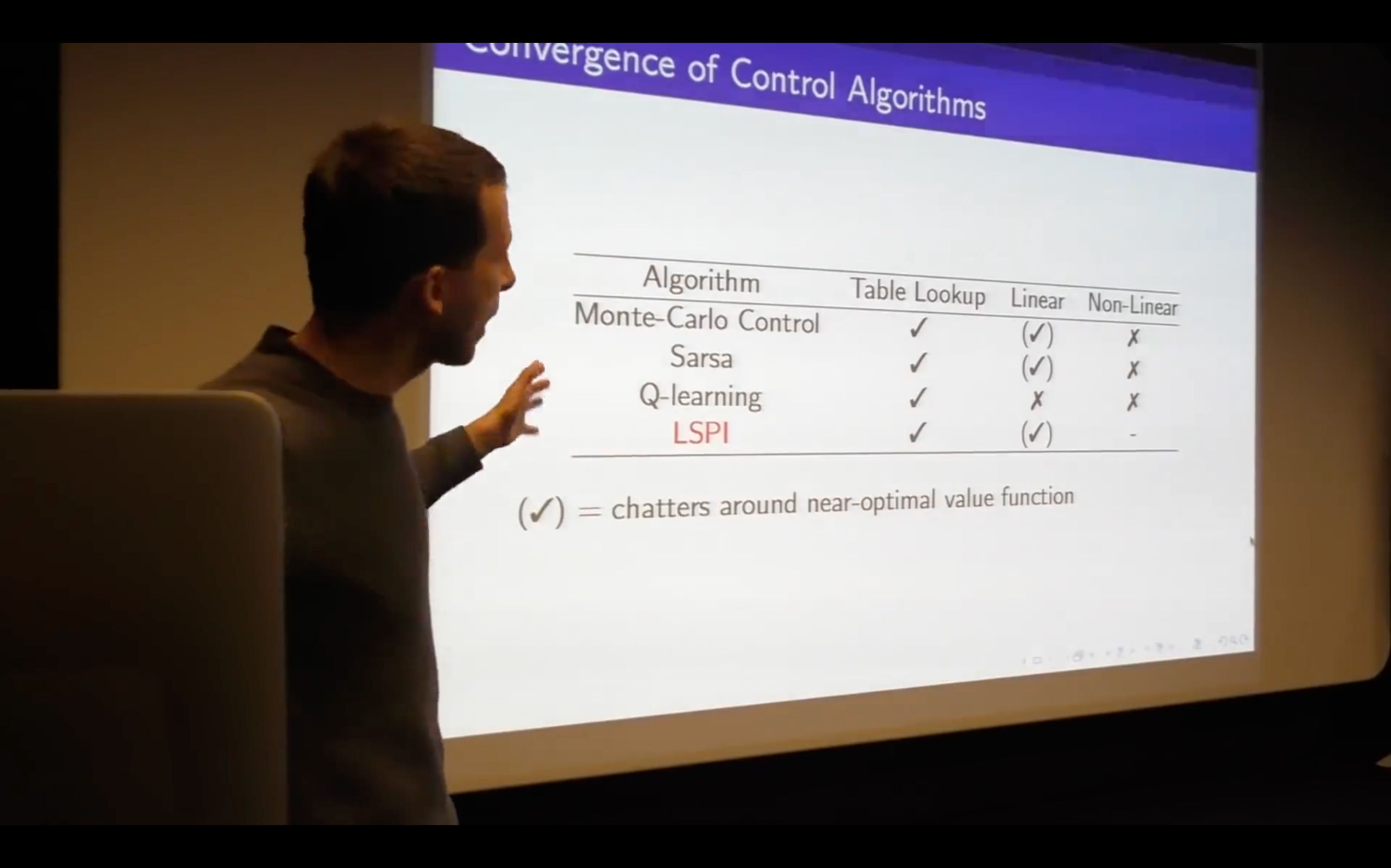
Lecture5: Model-Free Control
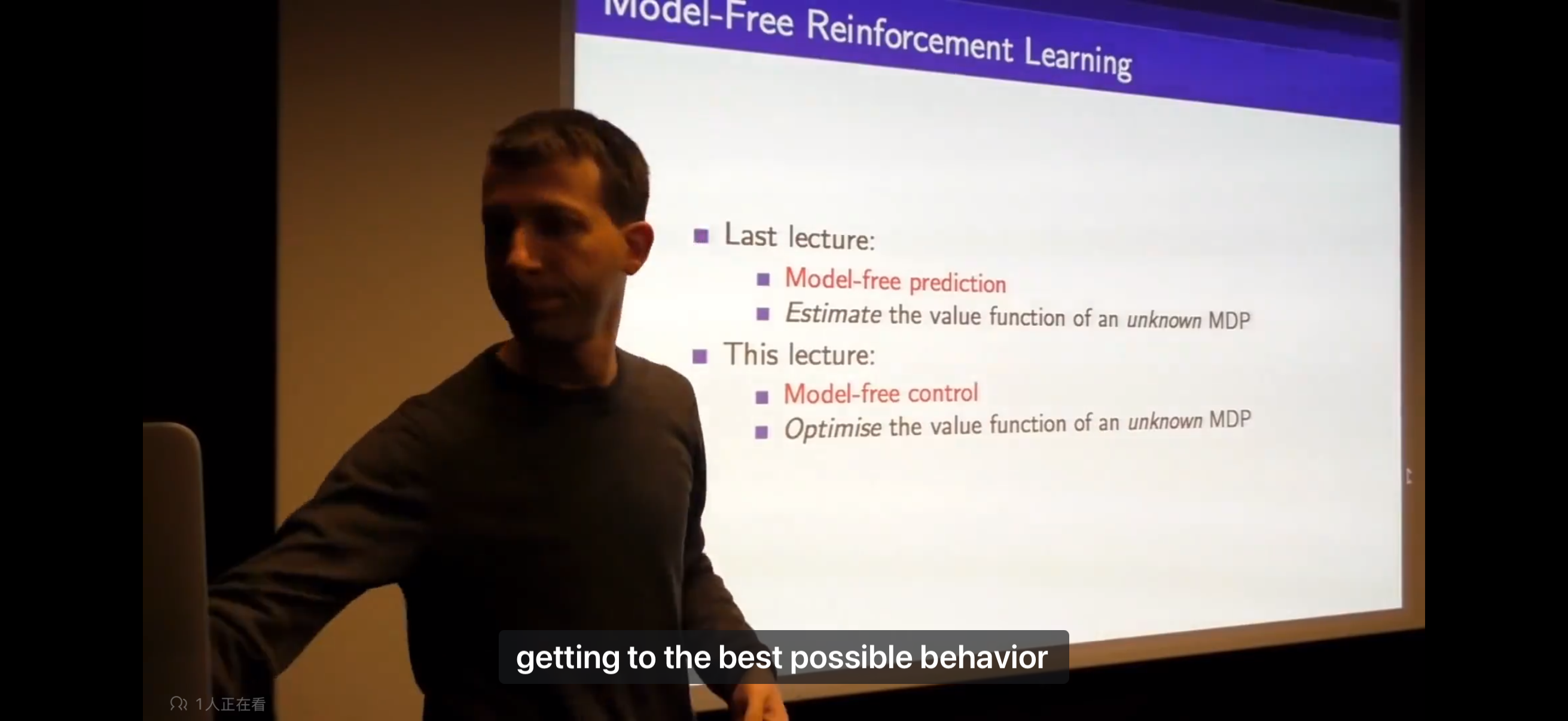
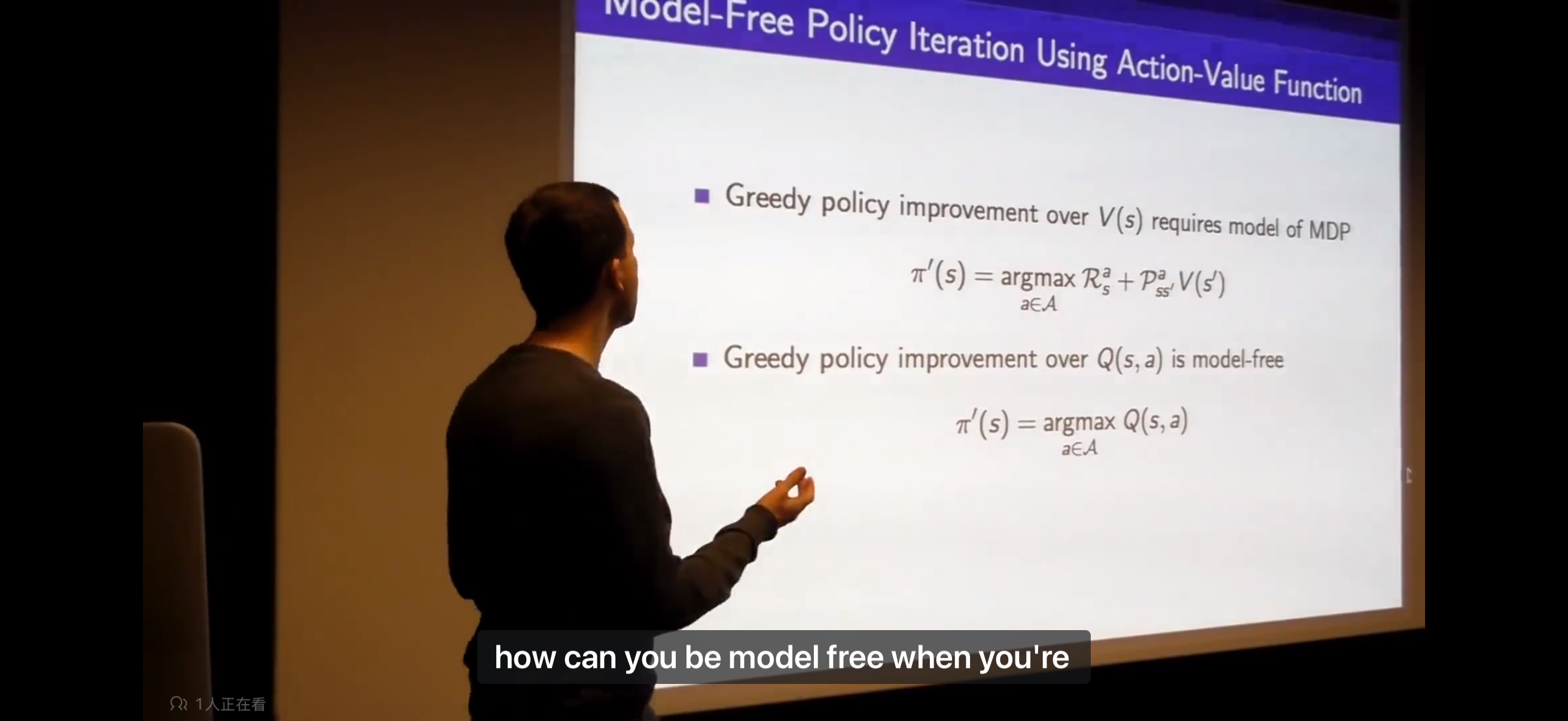
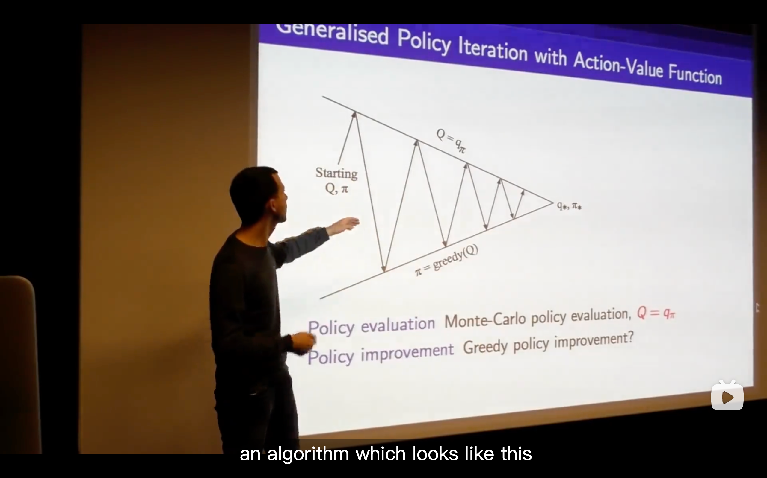
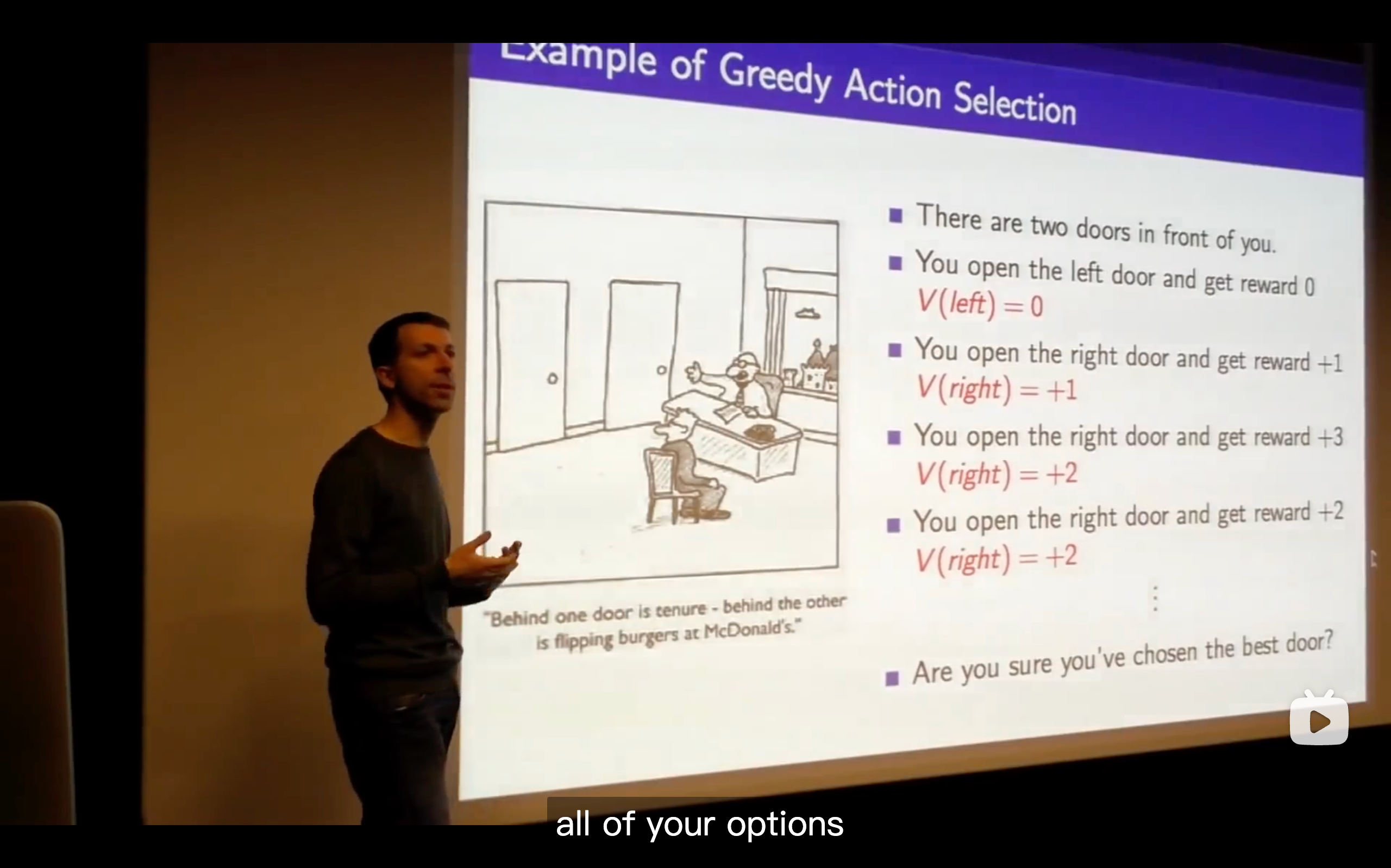
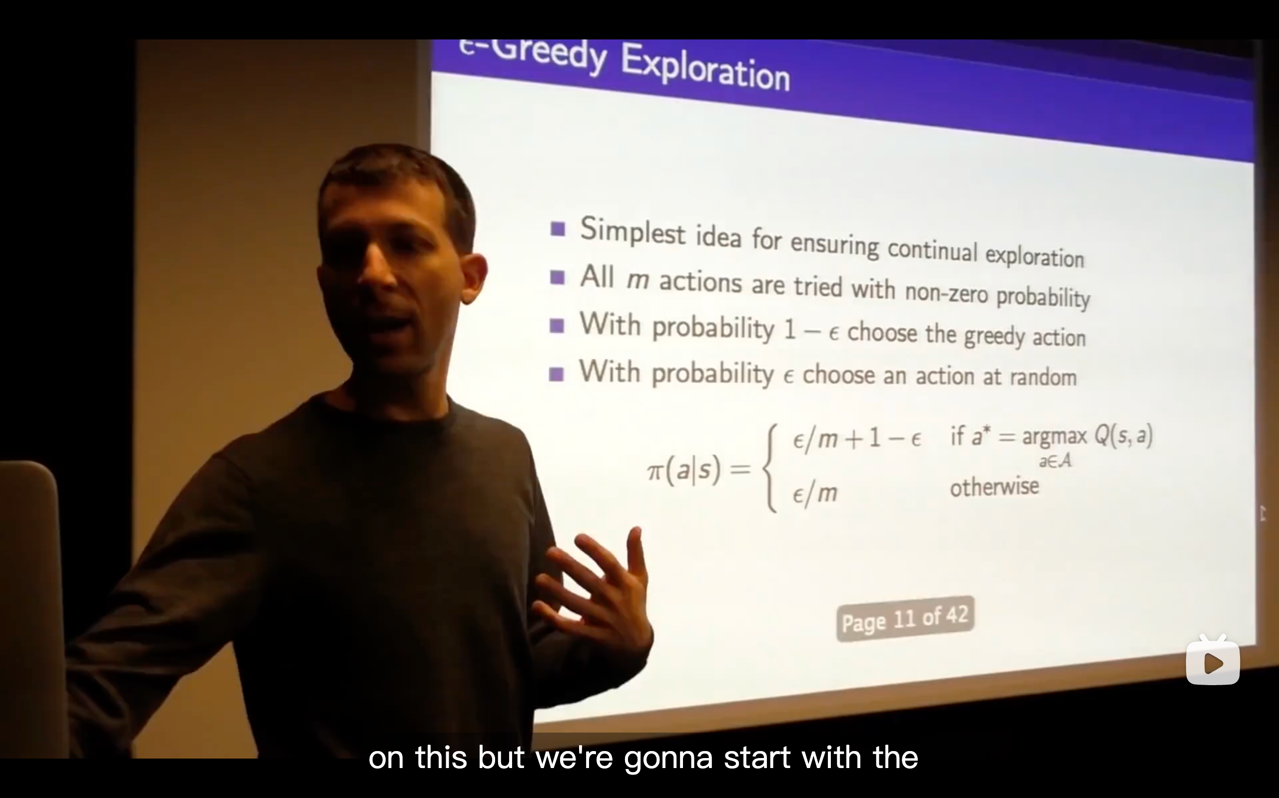
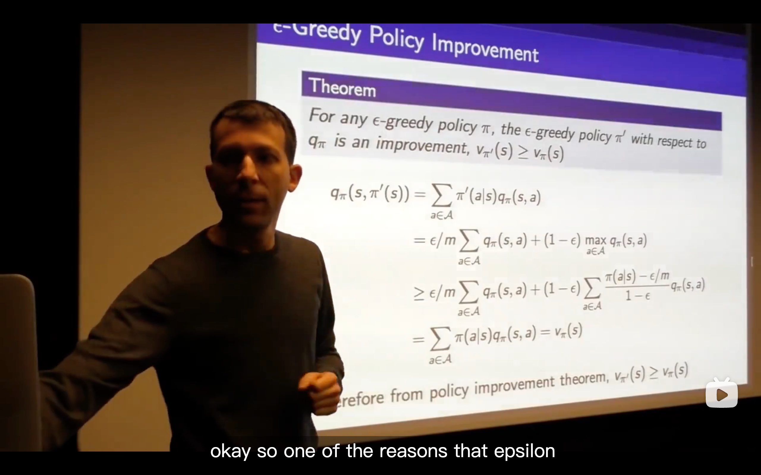
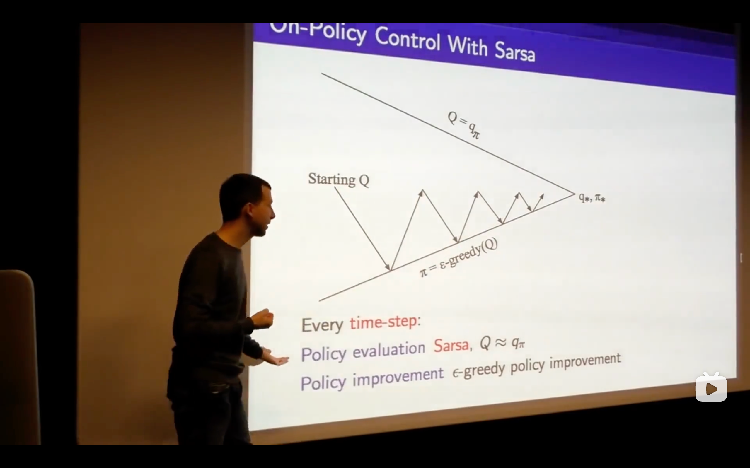
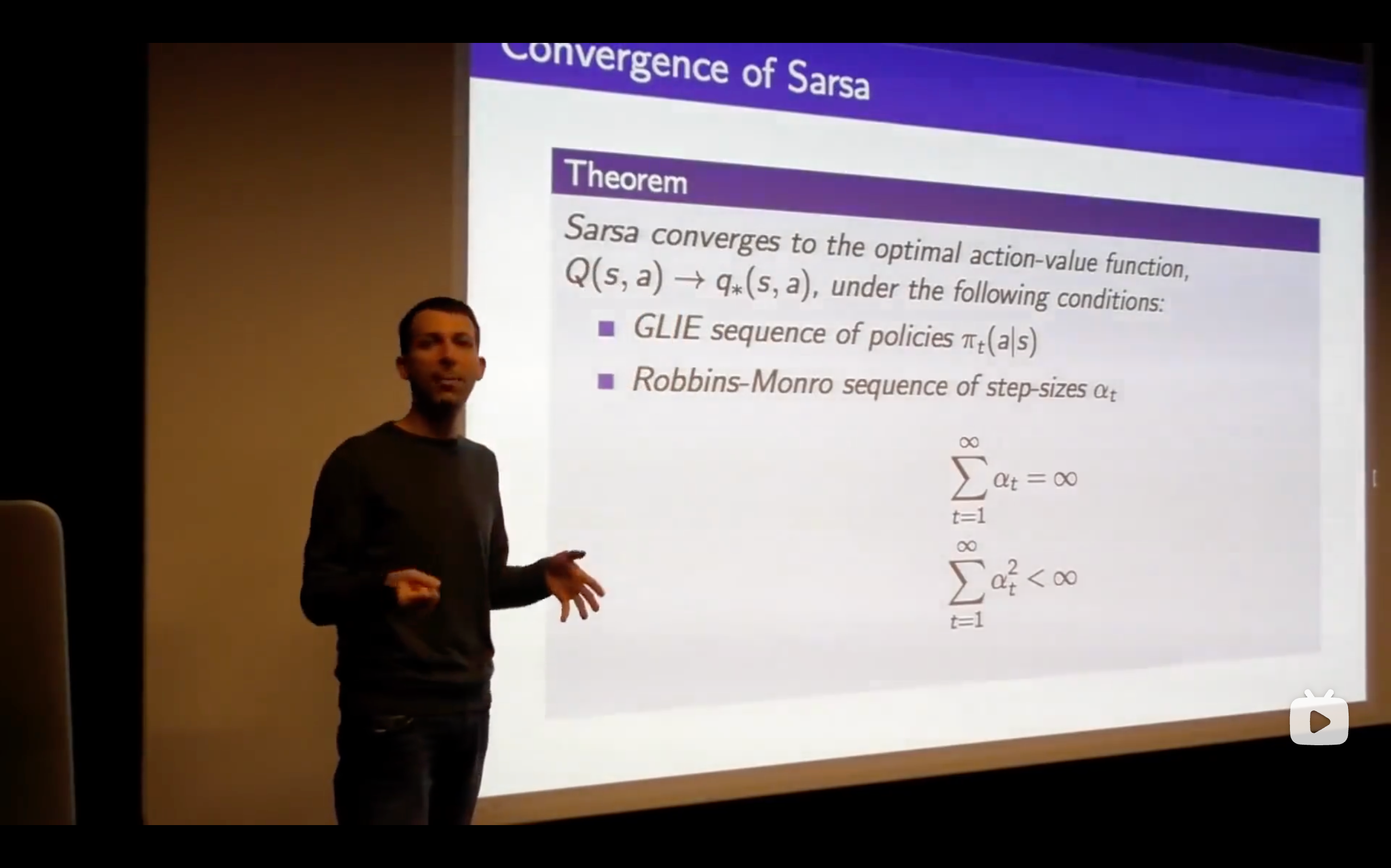
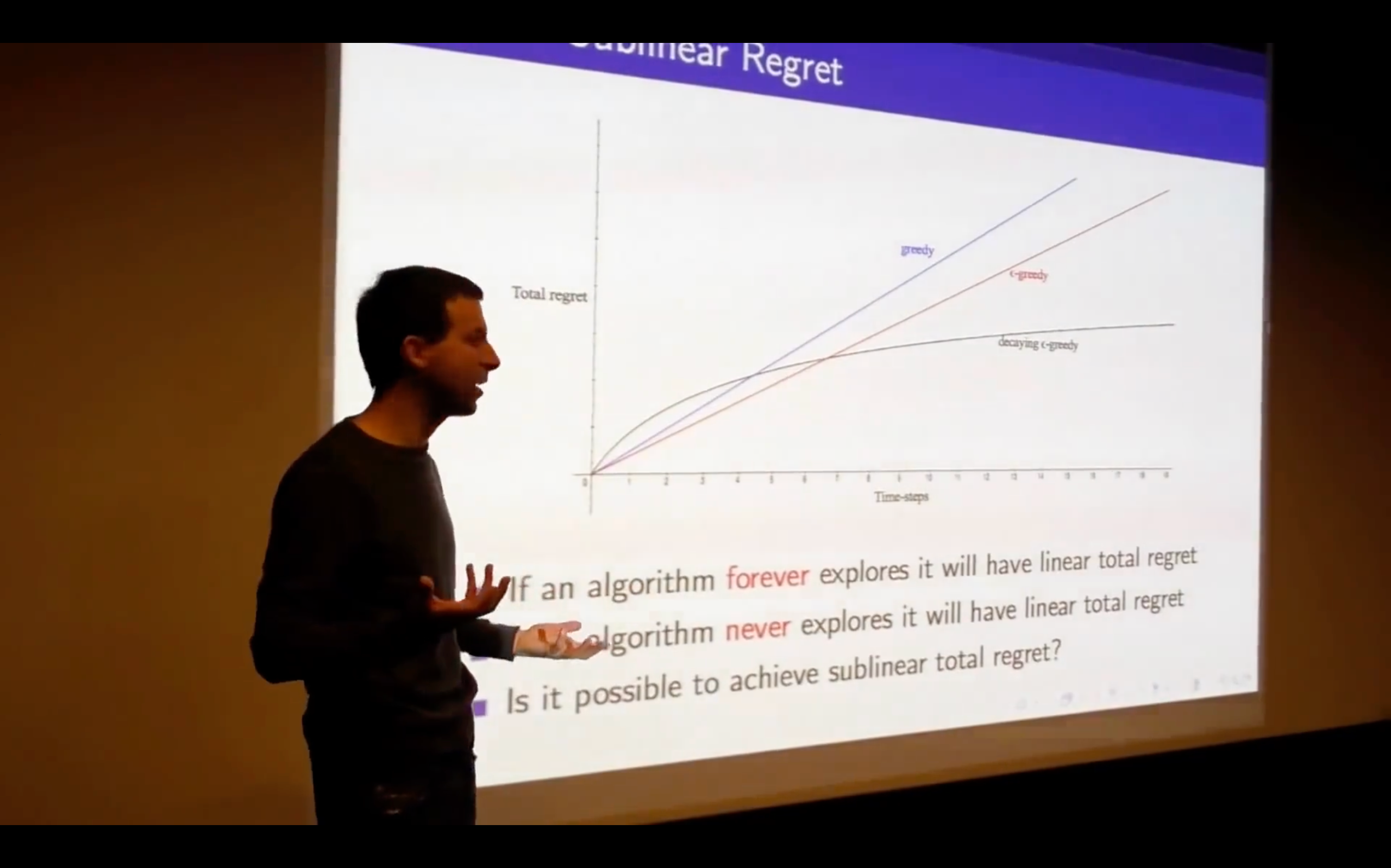
- You need to carry on exploring everything to make sure that you understand the the true value of all of your options. If you stop exploring certain actions, you can end up making incorrect decisions, getting stuck in some local incorrect optimum showing that your beliefs can be incorrect.
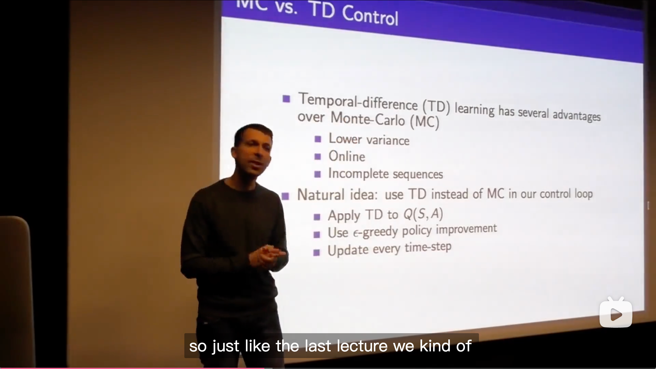
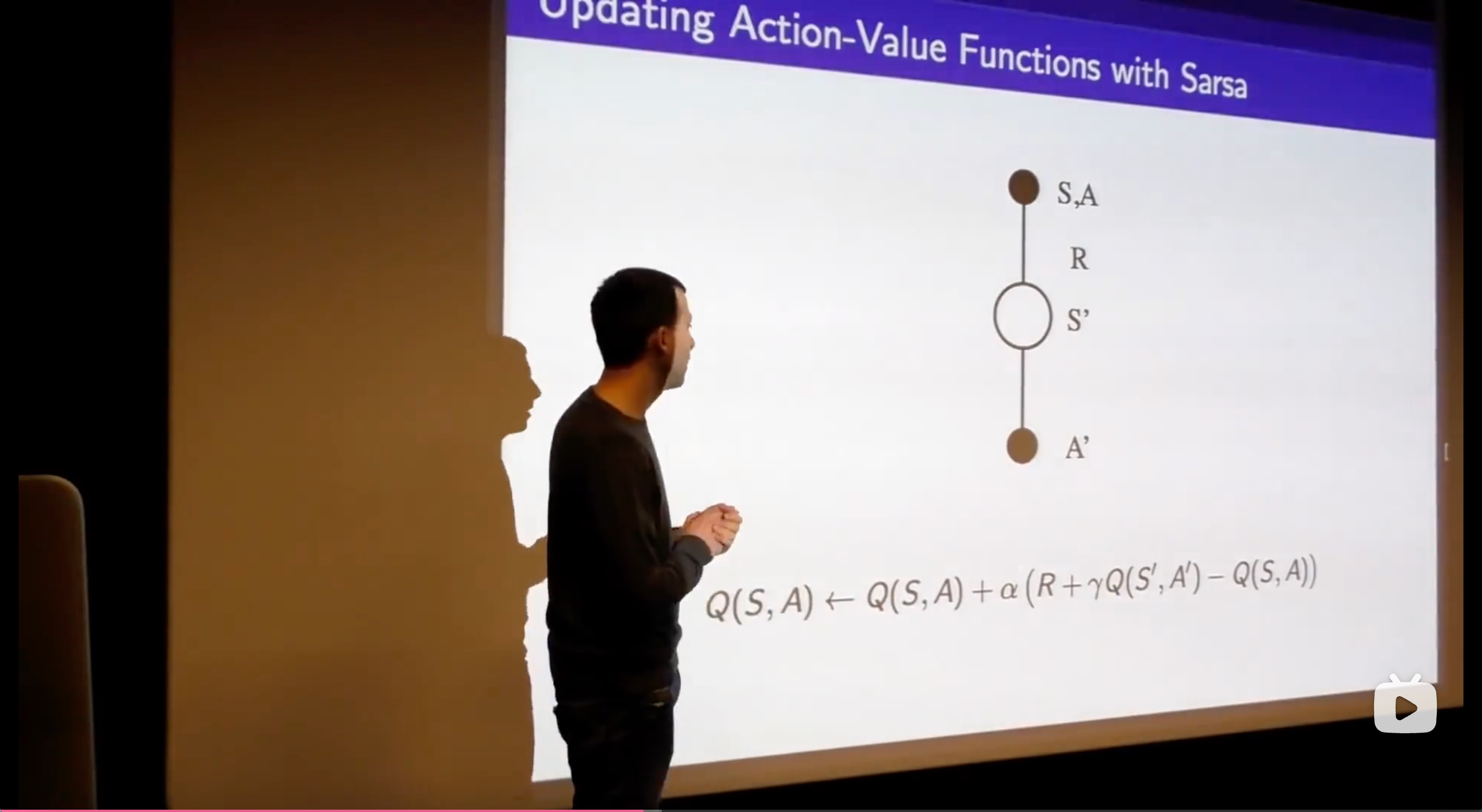
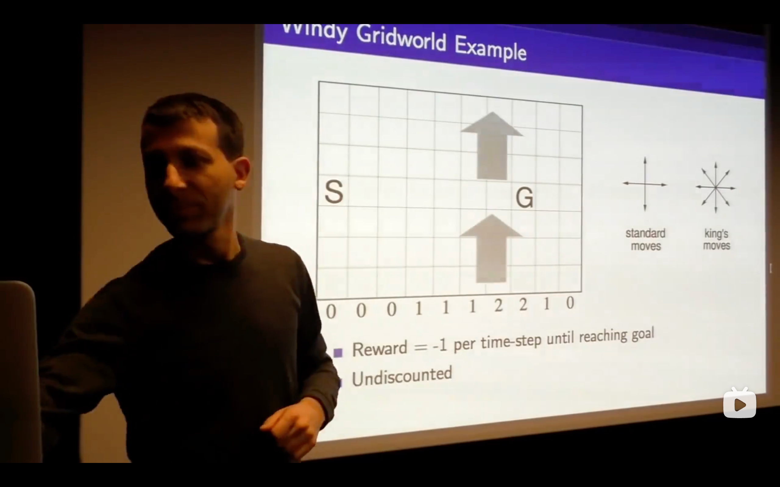
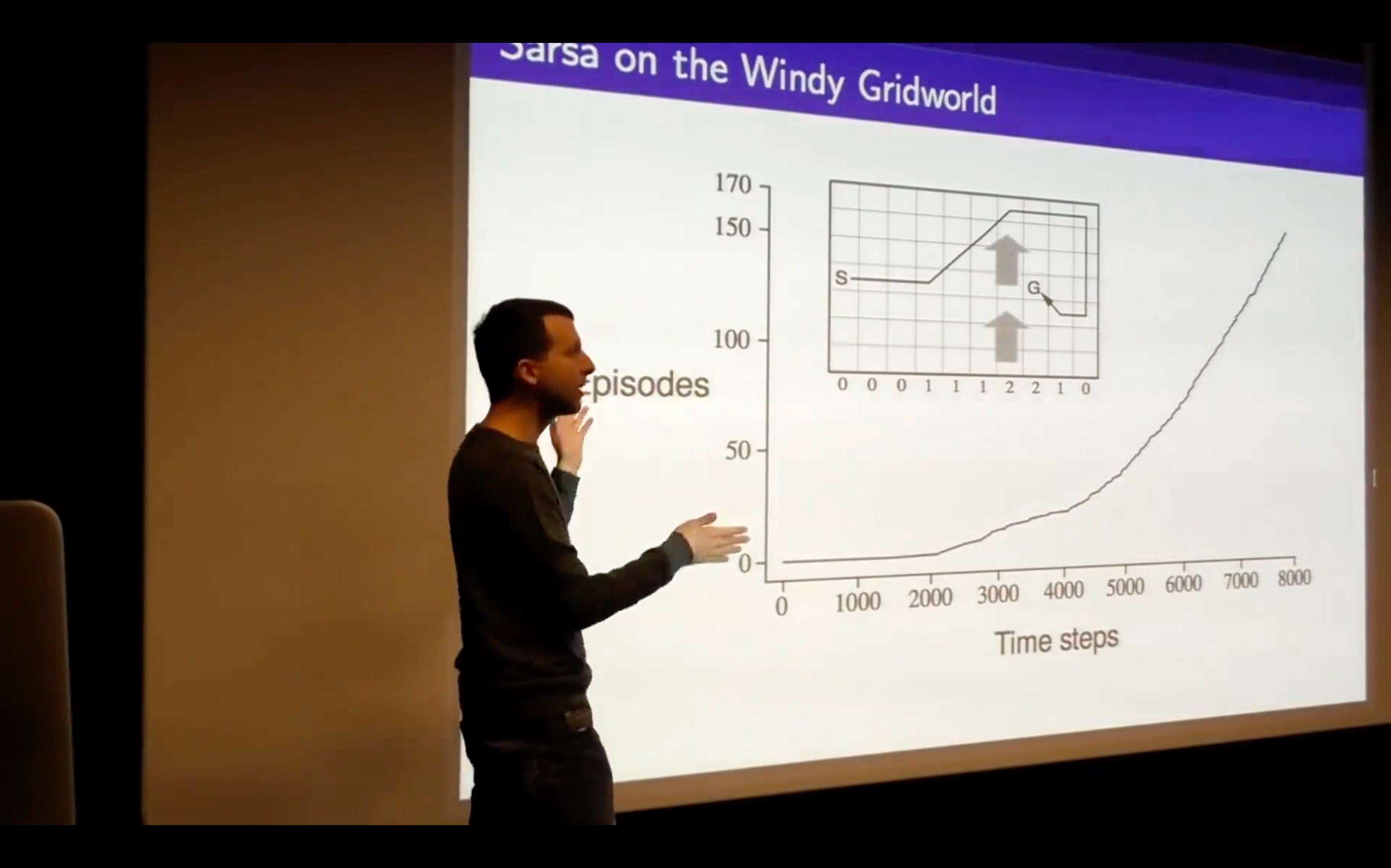
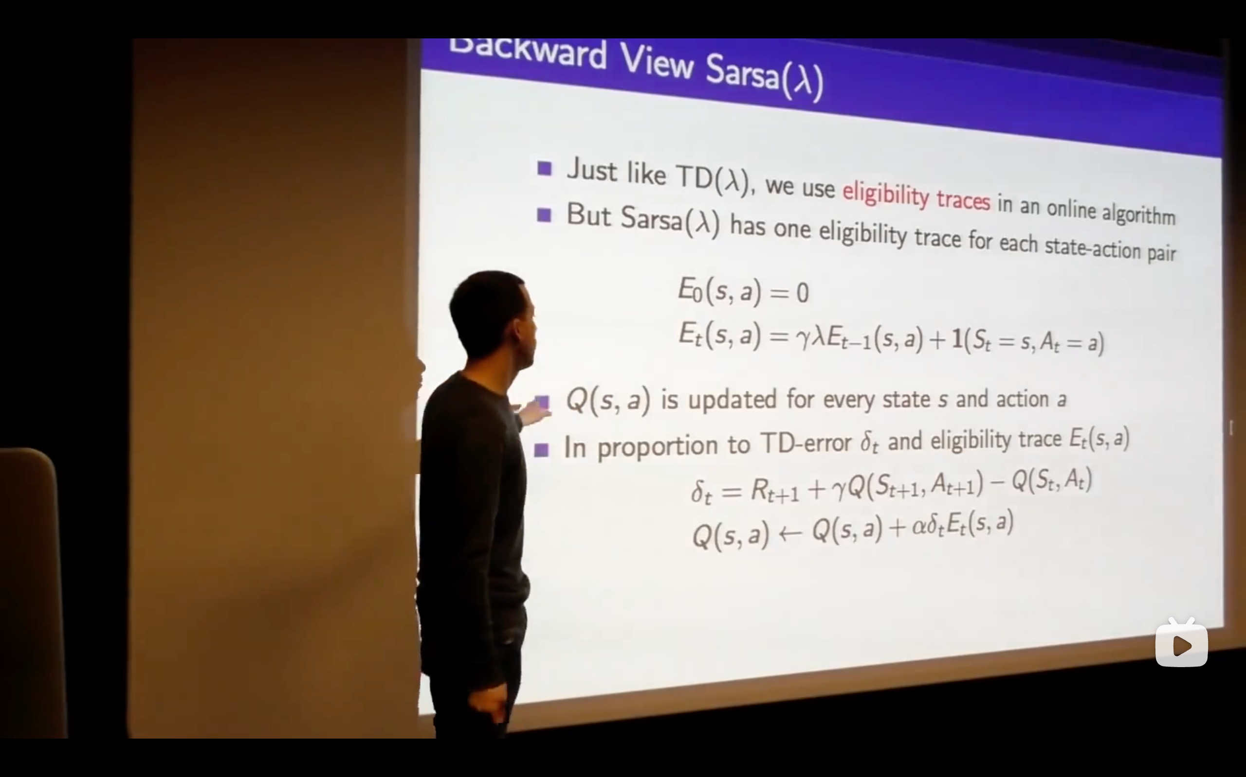
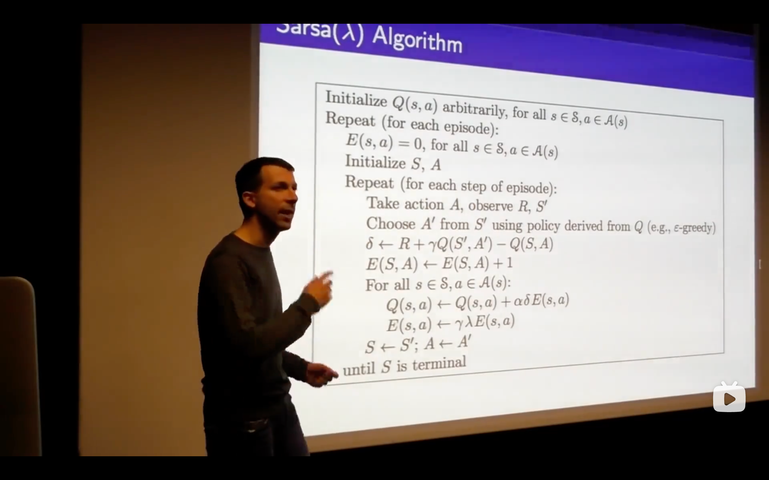
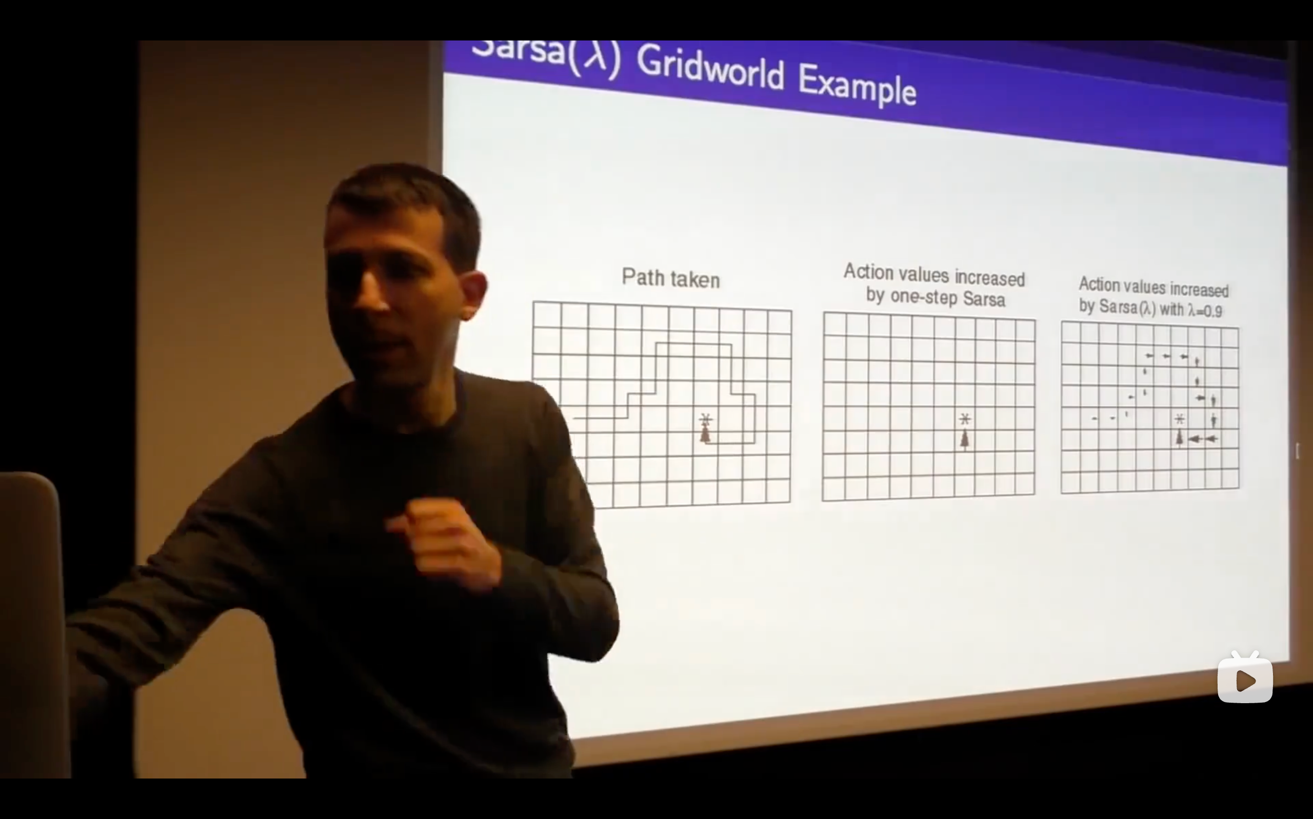
- Sarsa: State-Action-Reward-State-Action
- What's the problem of this?
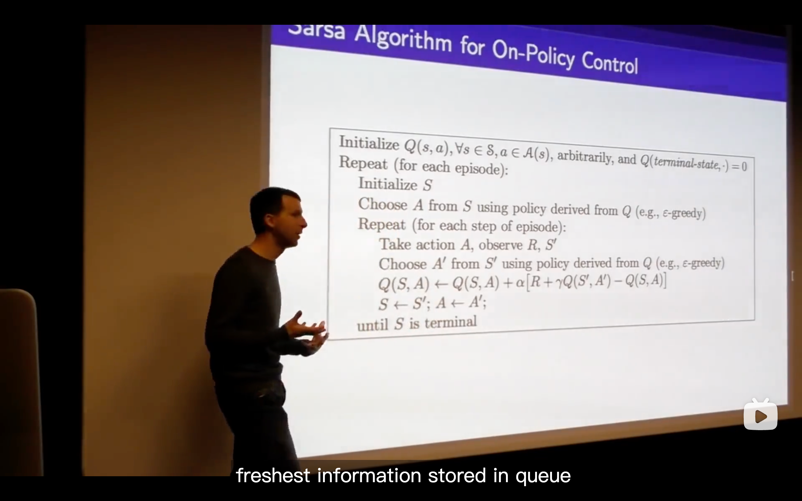
- This isn't an online algorithm, it's not something where we can take one step, update our Q-vlaue and immediately improve our policy, but we would like to be able to run things online and be able to get the freshest possible updates ,then updating immediately.
https://chat.qwen.ai/s/t\_53c20bd8-dfc6-4204-886f-74ecba03690f?fev=0.1.9
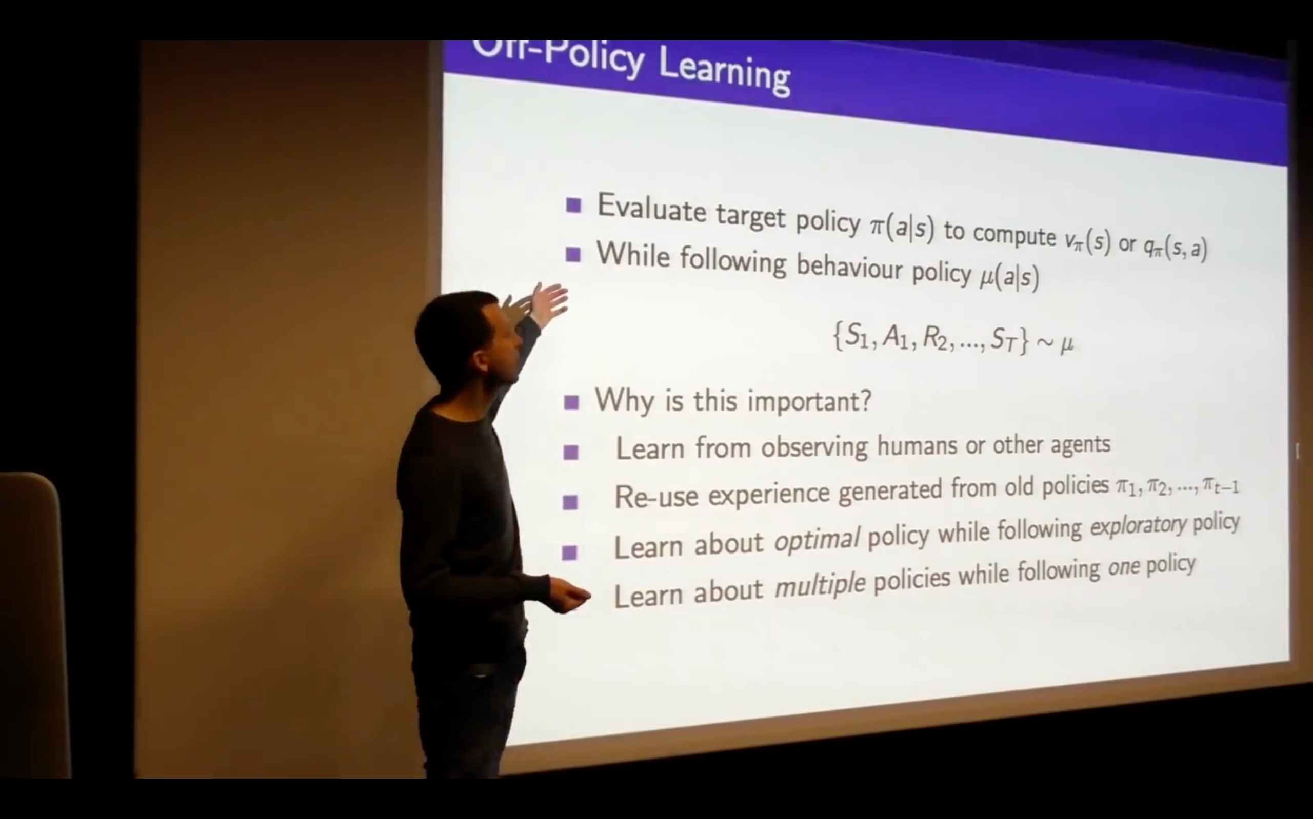
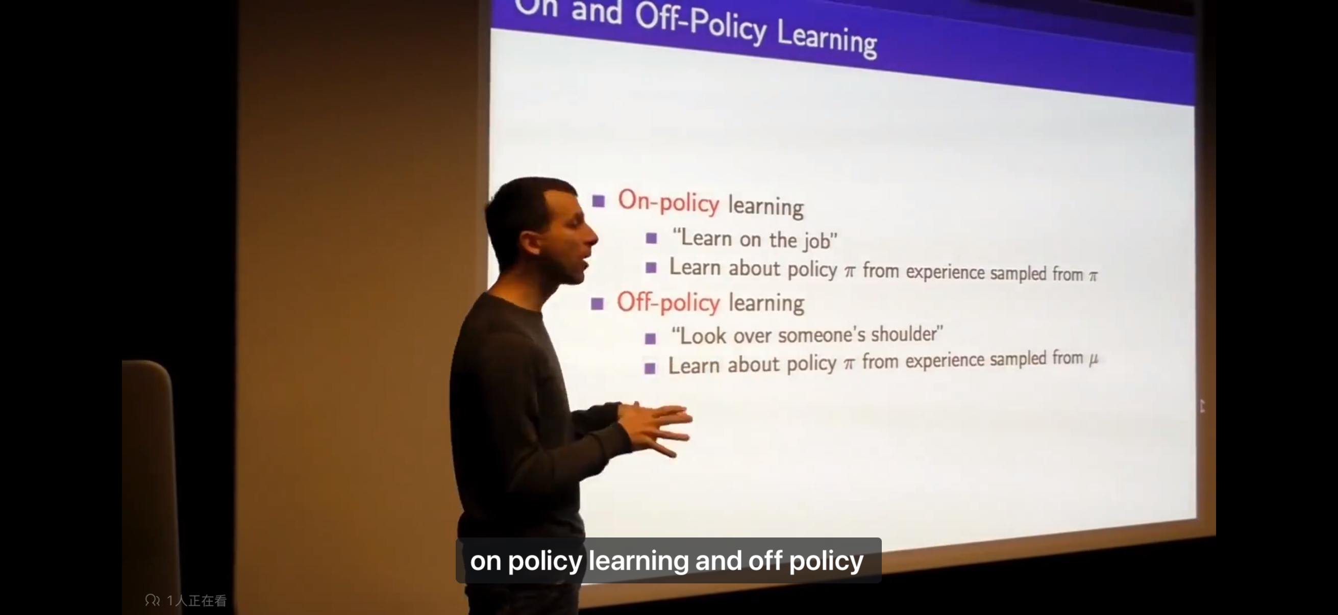
: Target Policy : Behaviour Policy
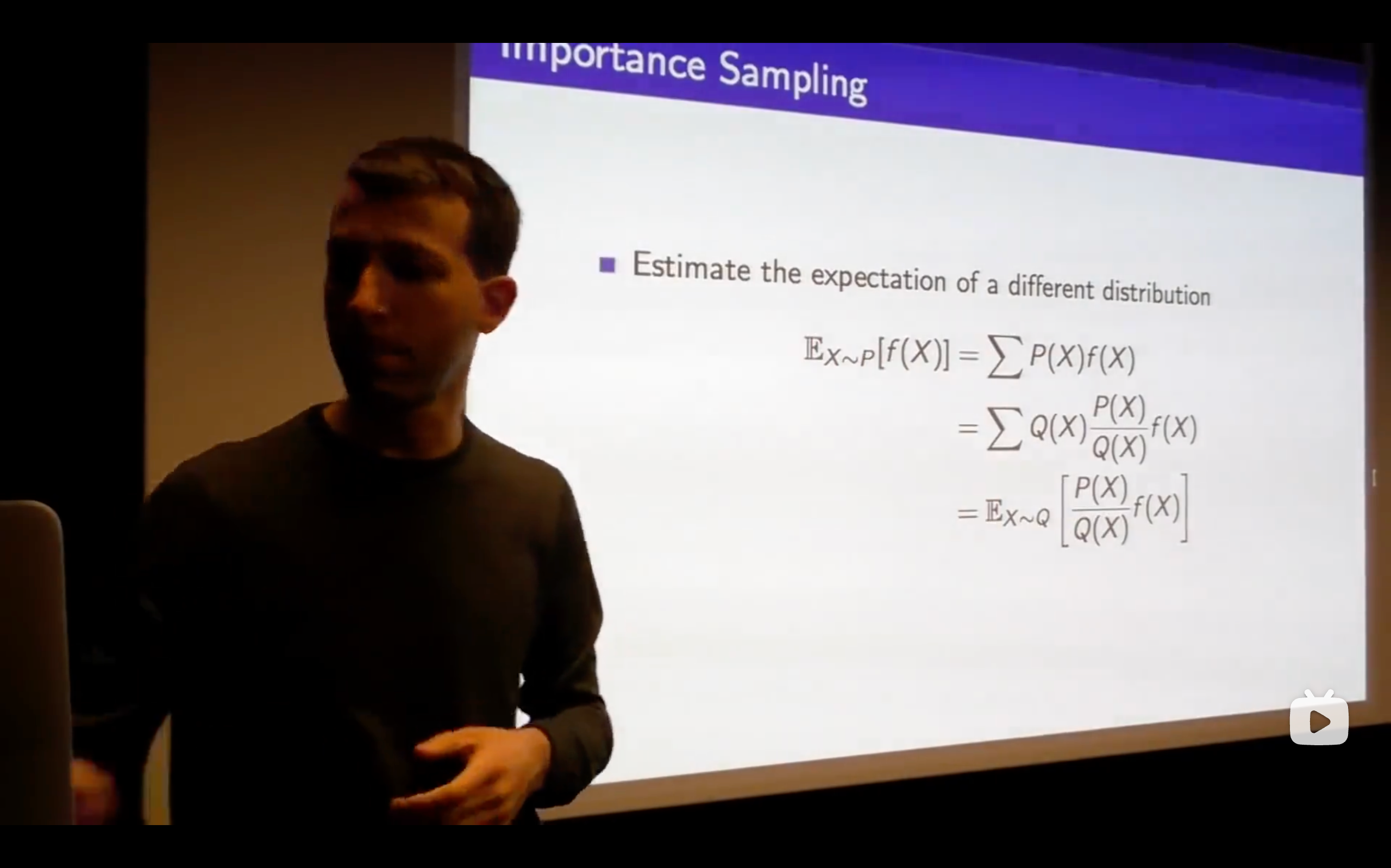
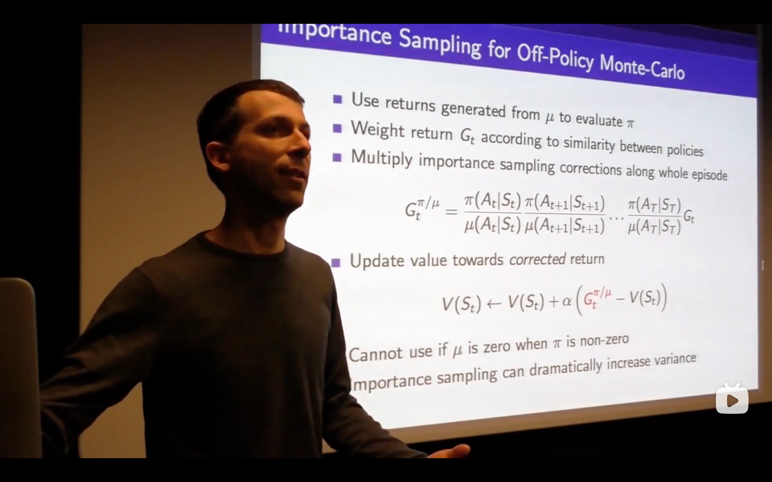
- Change P sampling into Q sampling.
- importance weight:
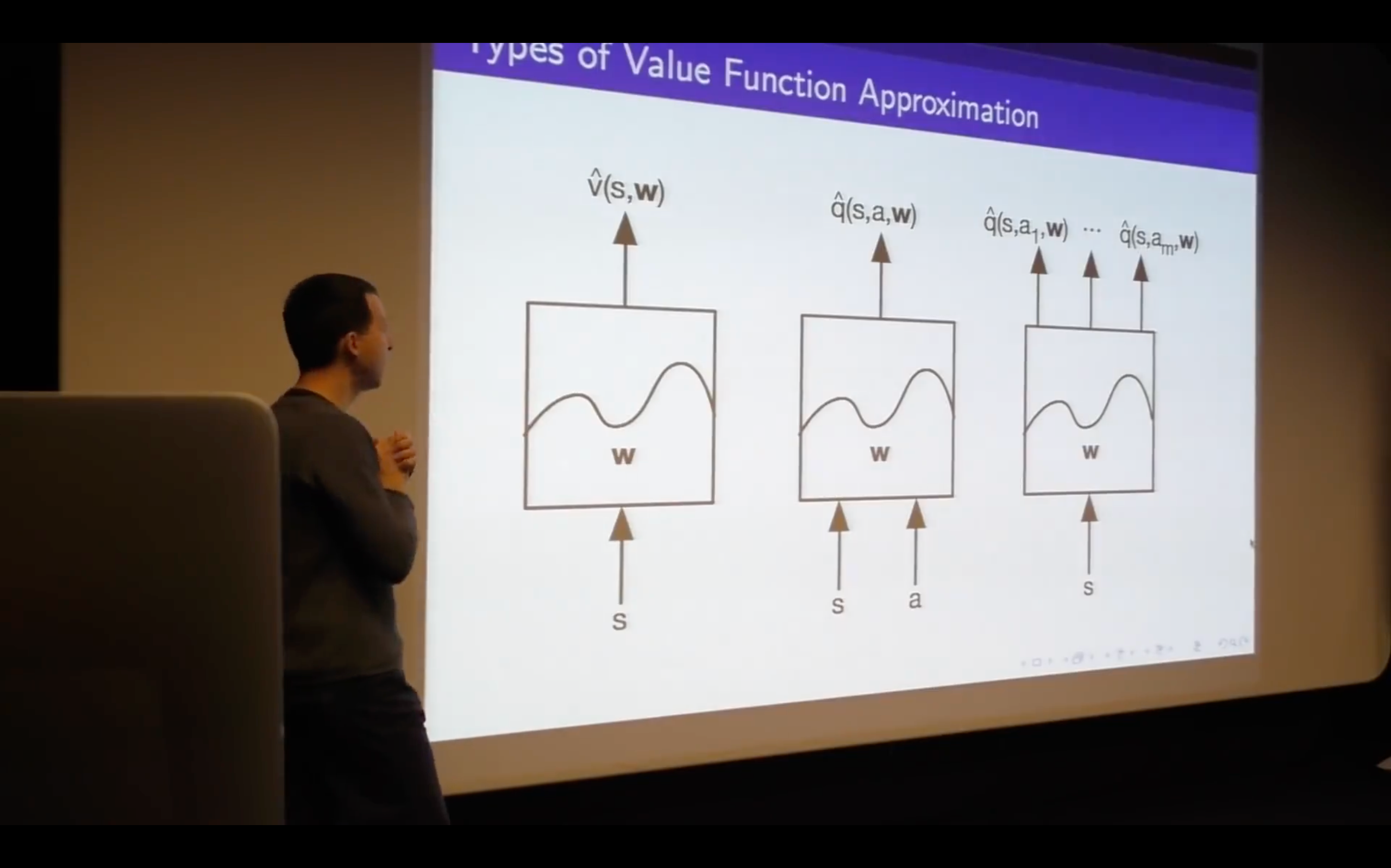
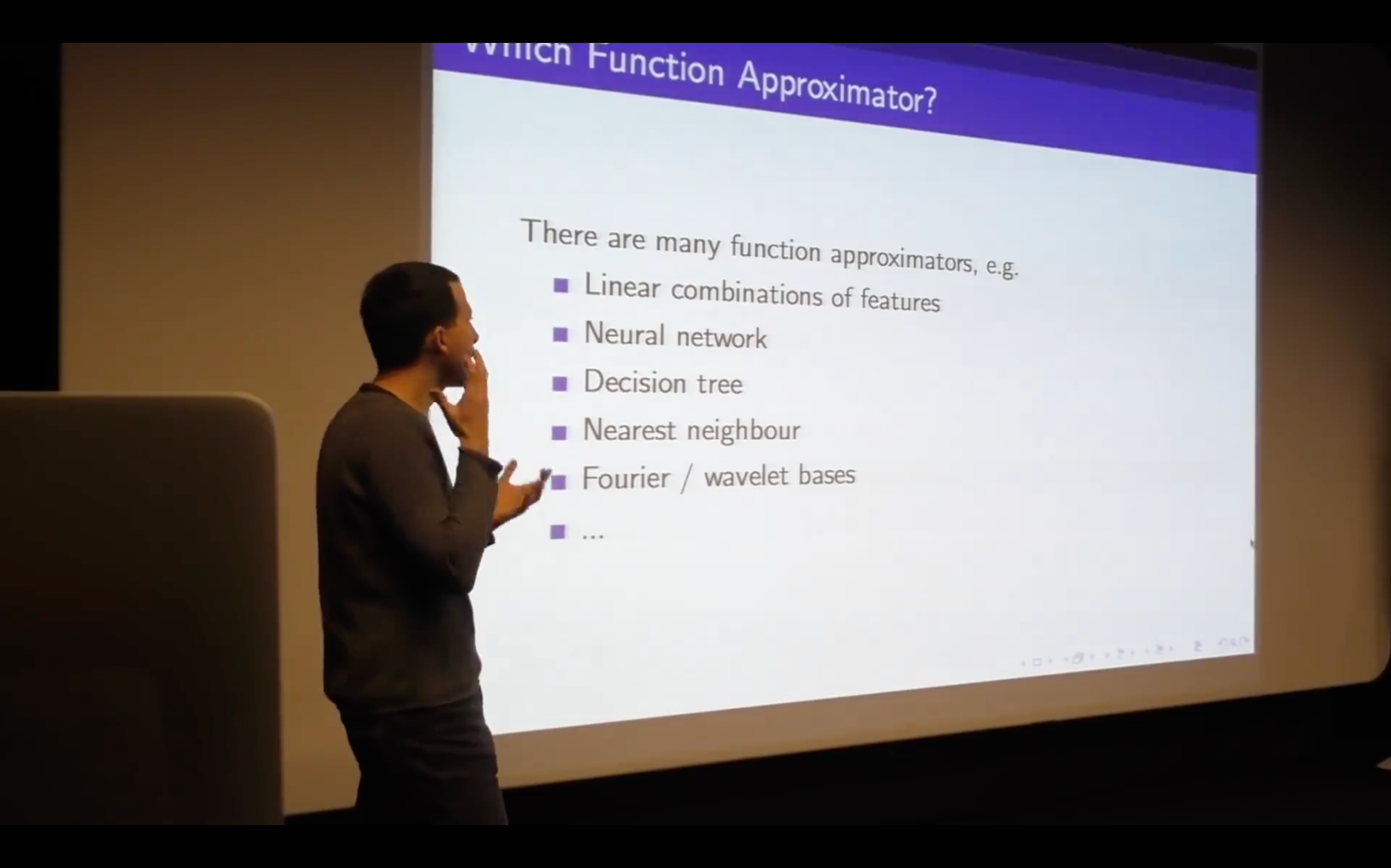
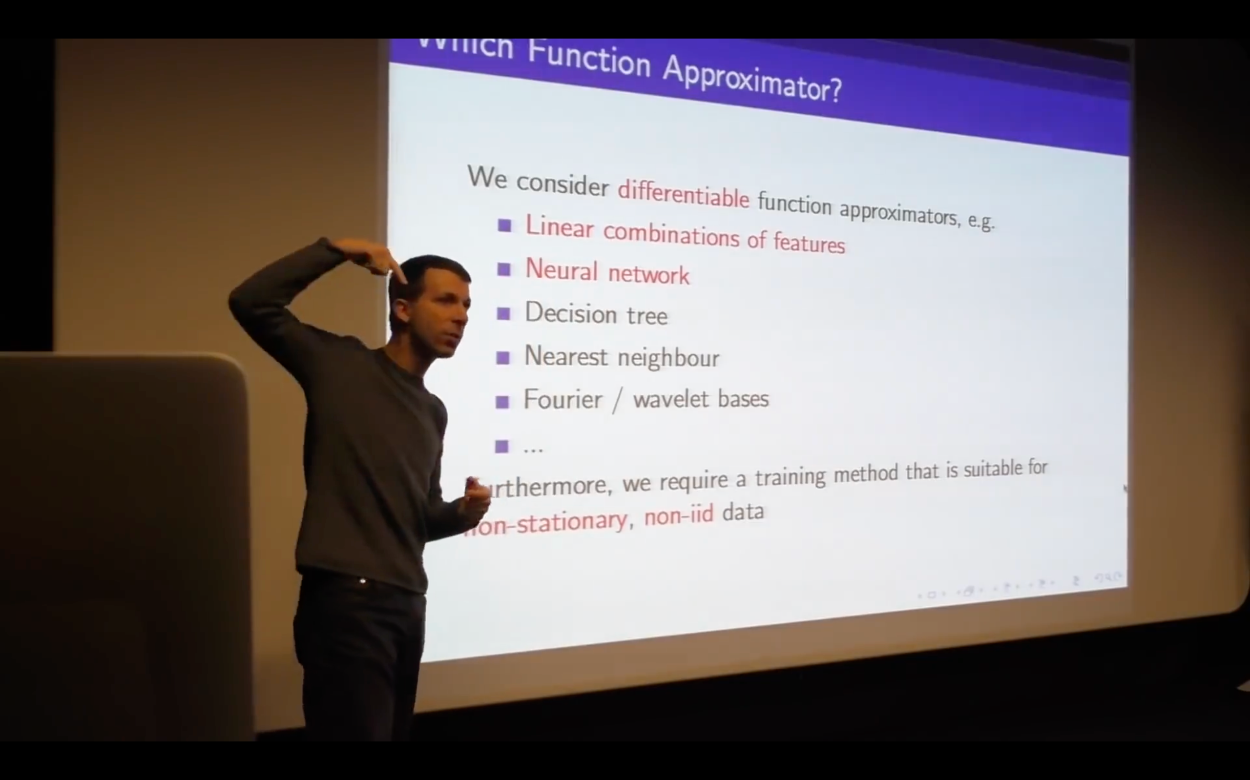
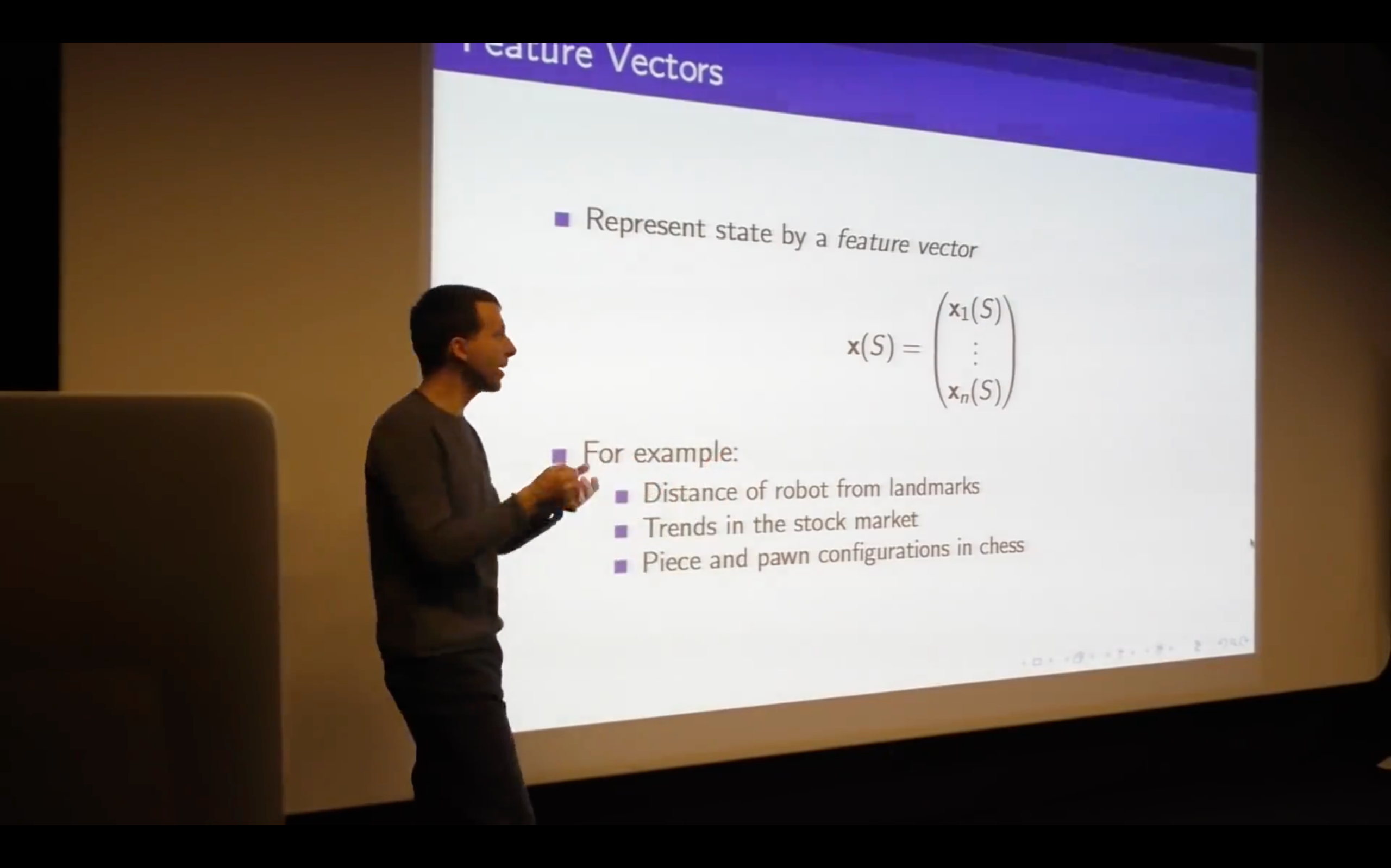
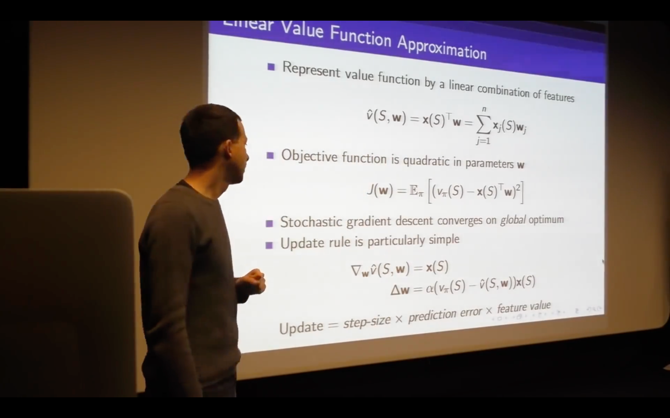
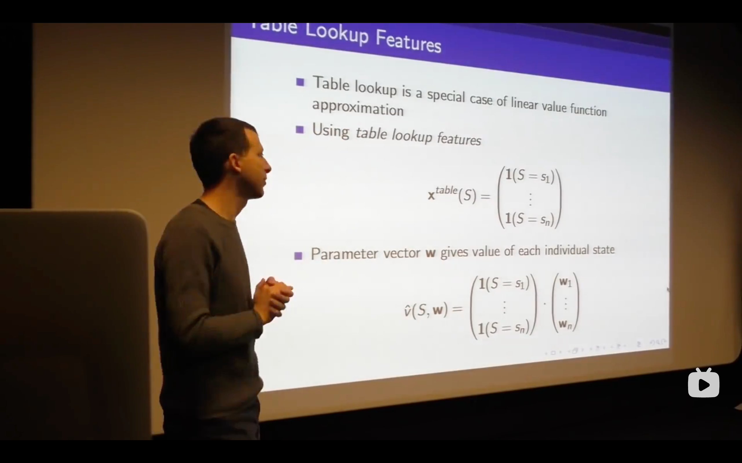
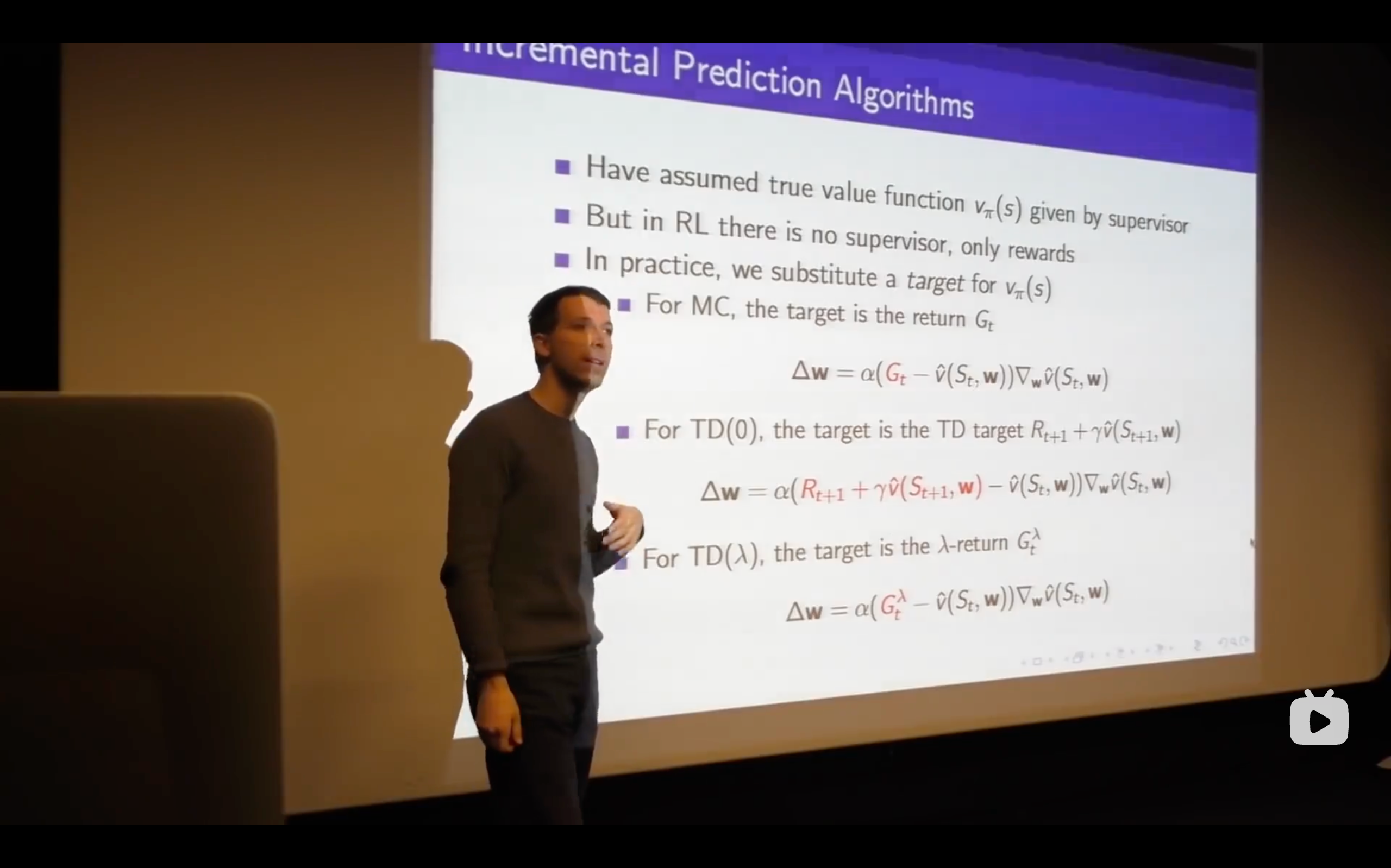
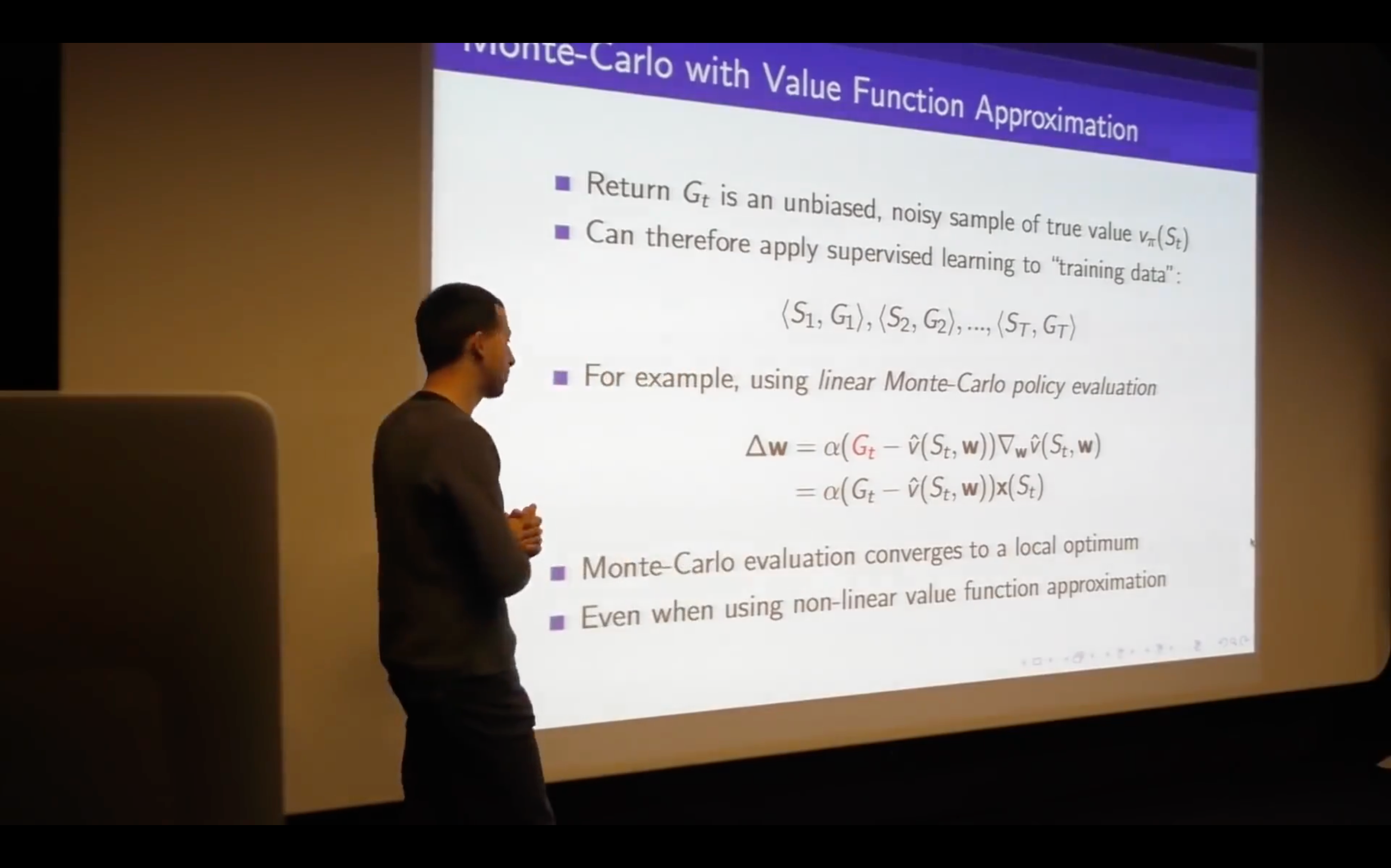
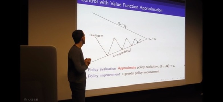
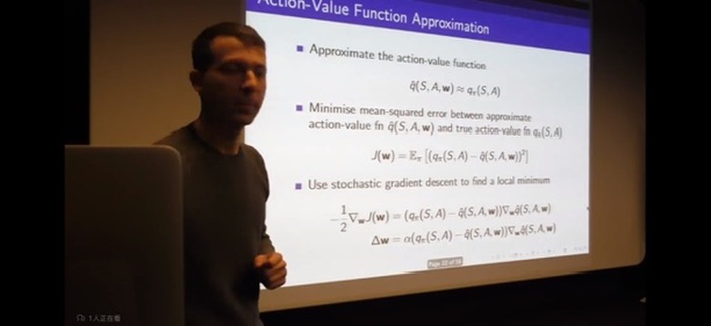
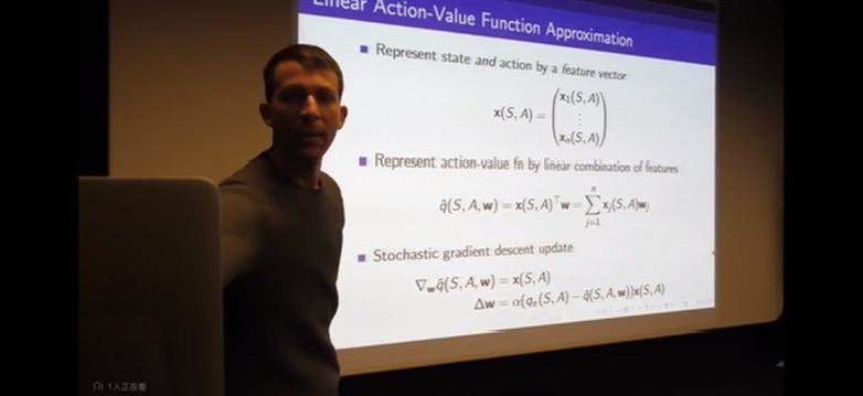
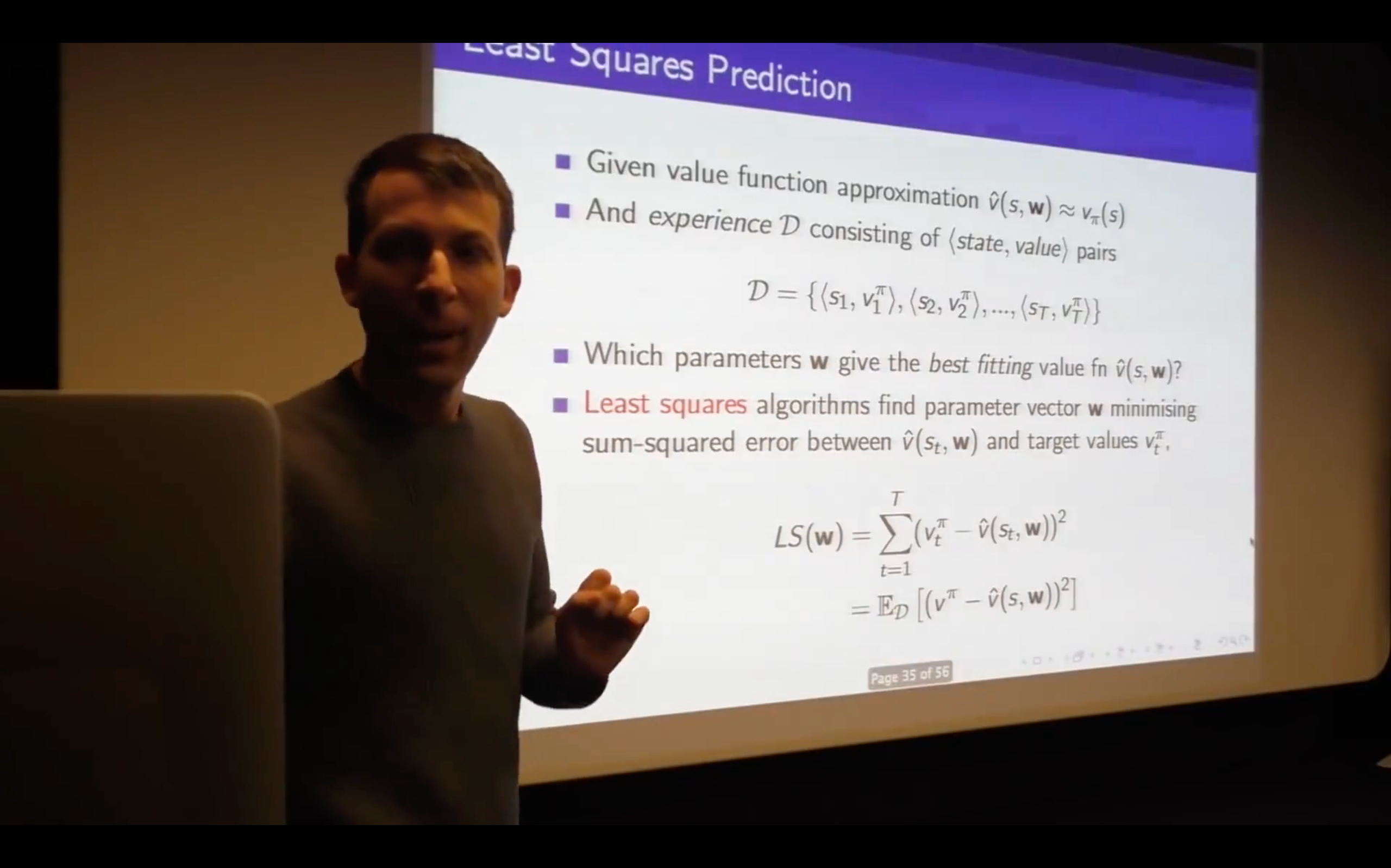
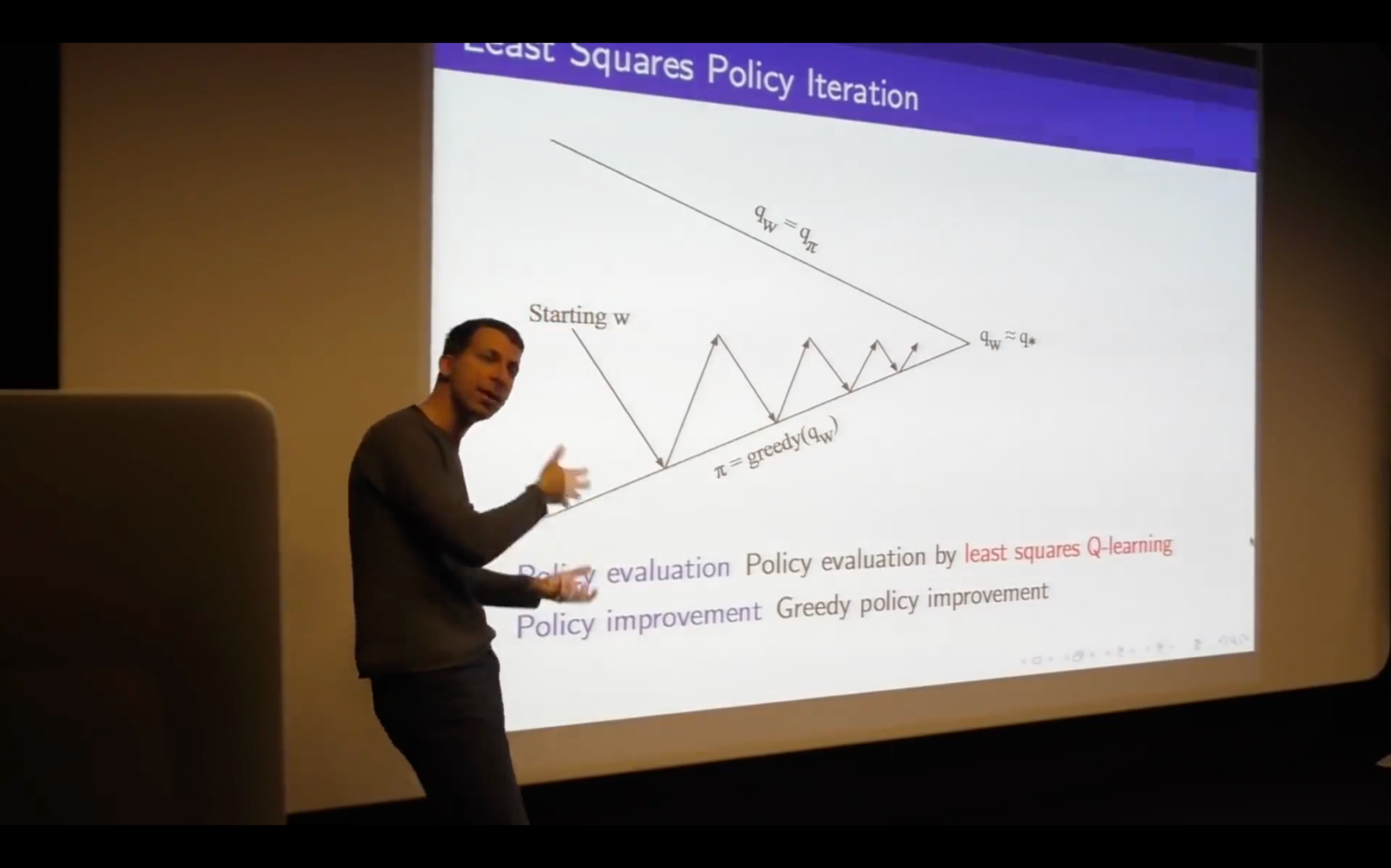
Lecture6: Value Function Approximation
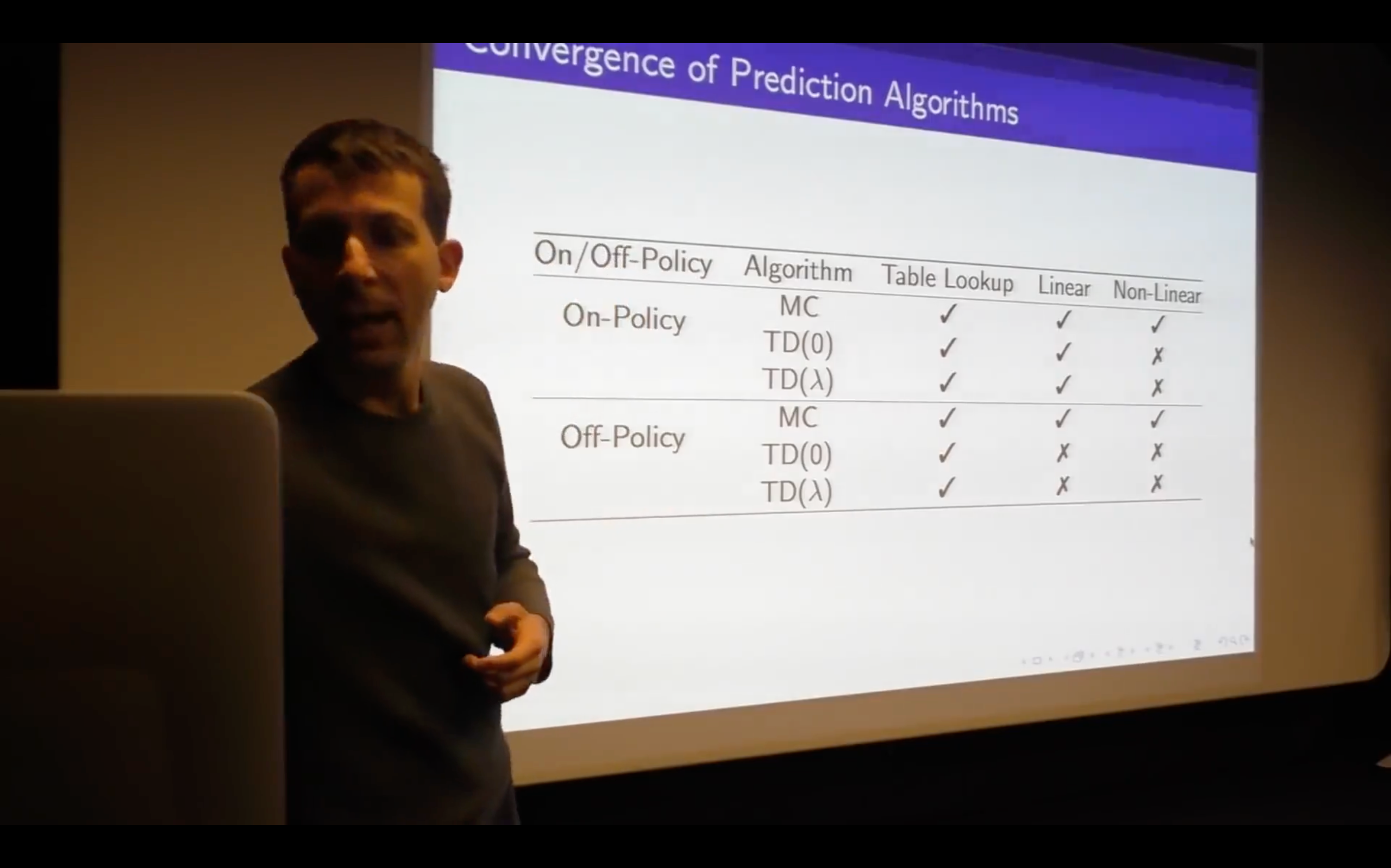
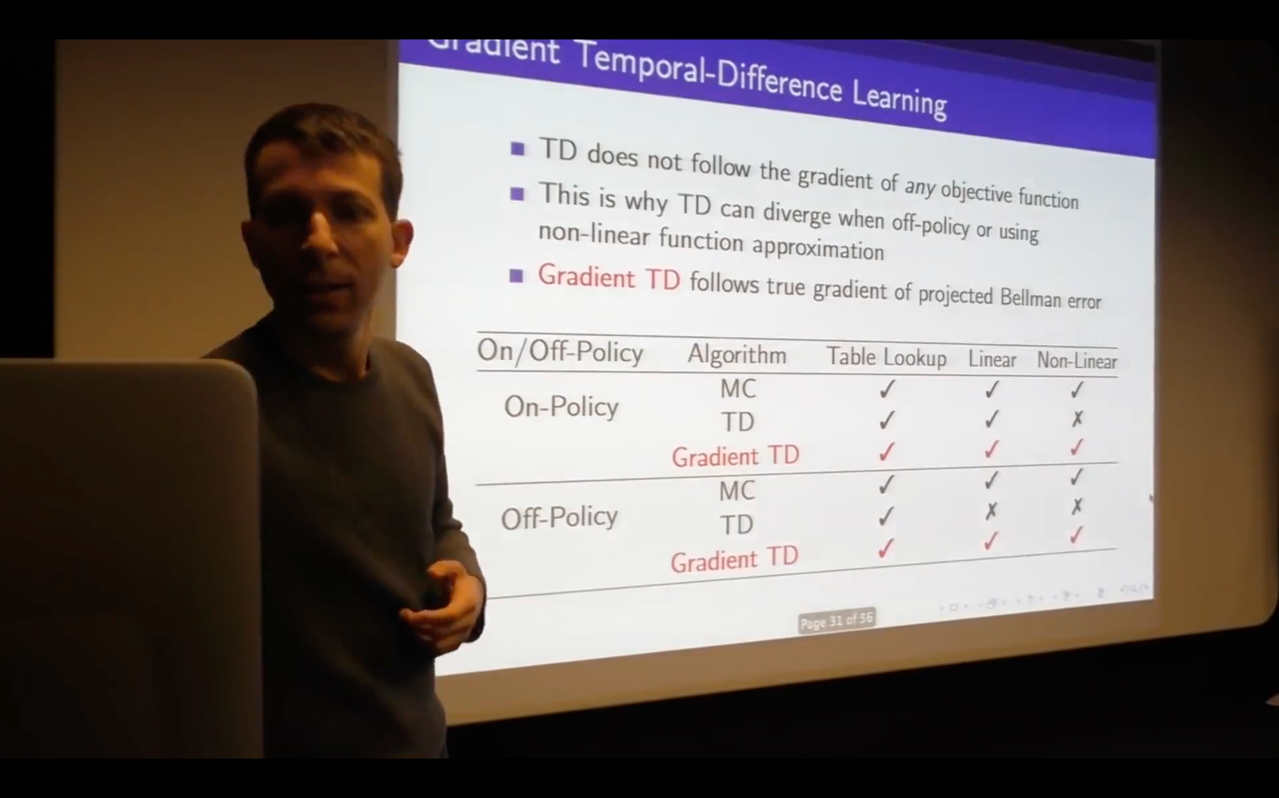
Introduction
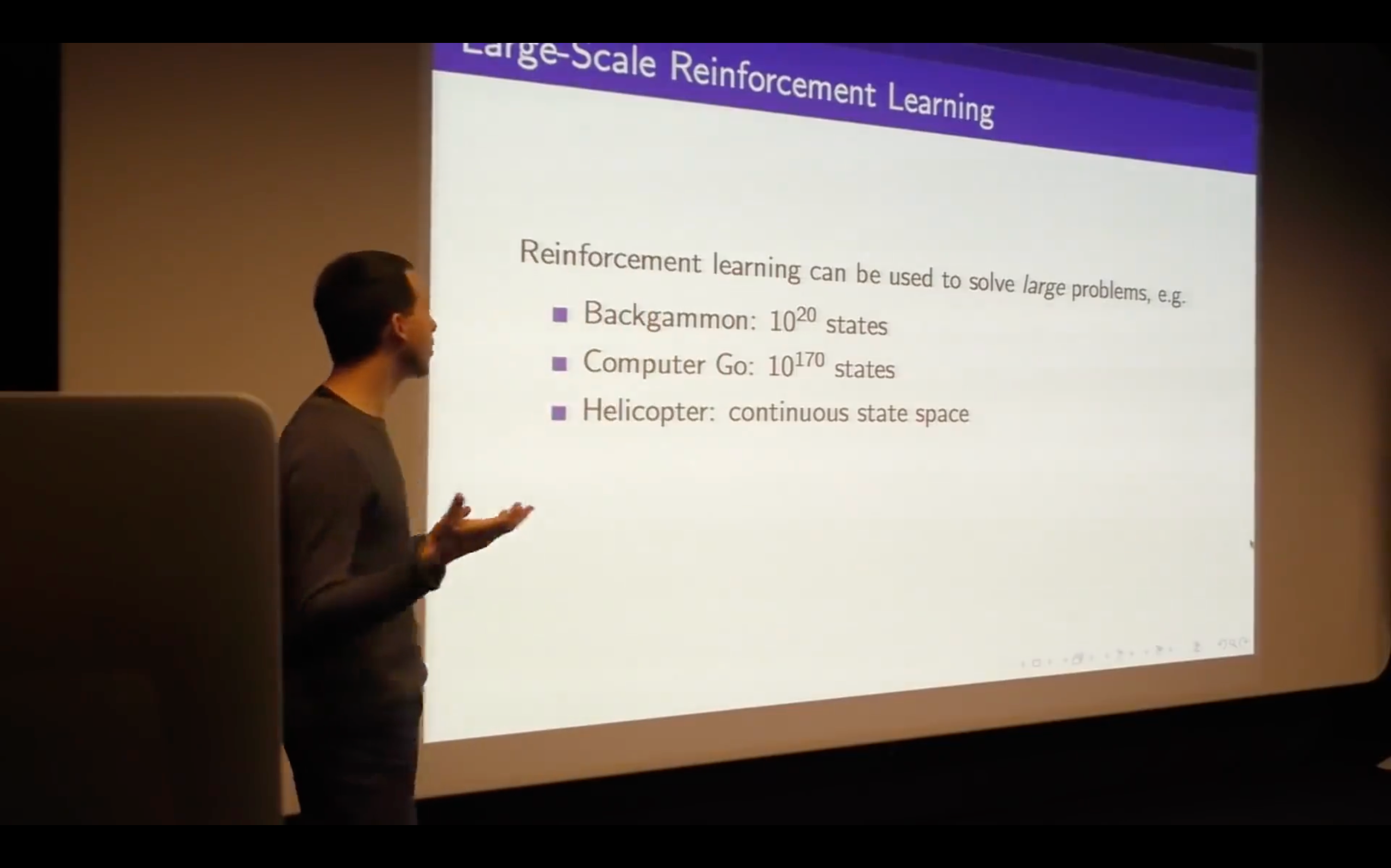
How can we scale up the model-free methods for prediction and control from the last two lectures?
What we'll do is not just reduce the memory but also allow us to generalize -- to fit our function to approximate our states that we've never seen.
- Consider this action here, how could that be?
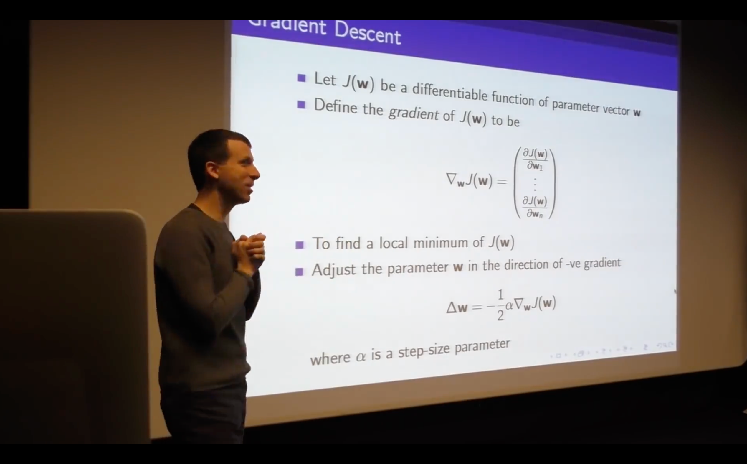
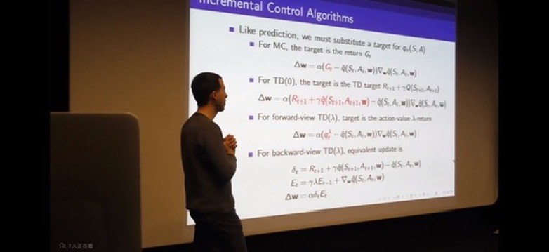
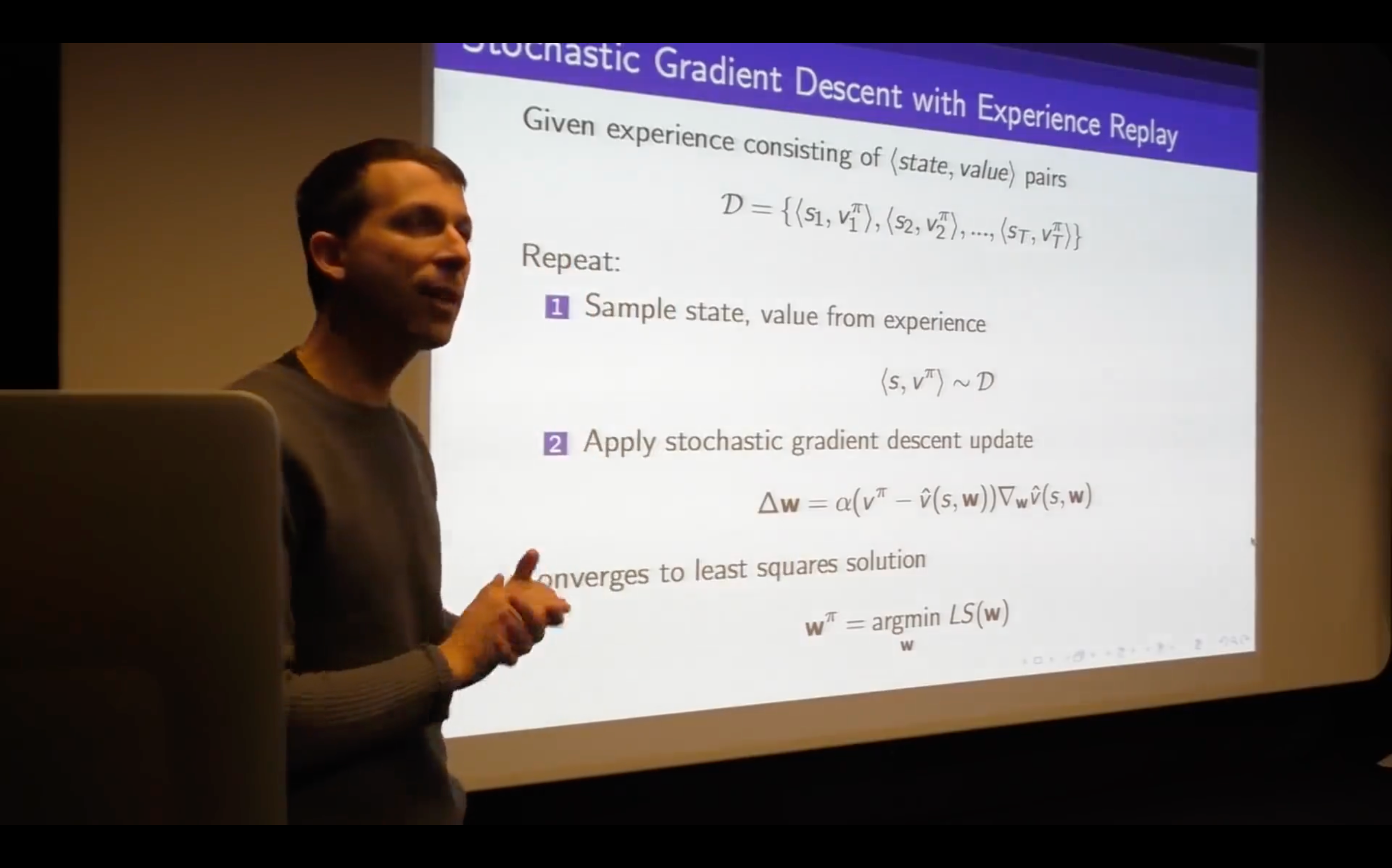
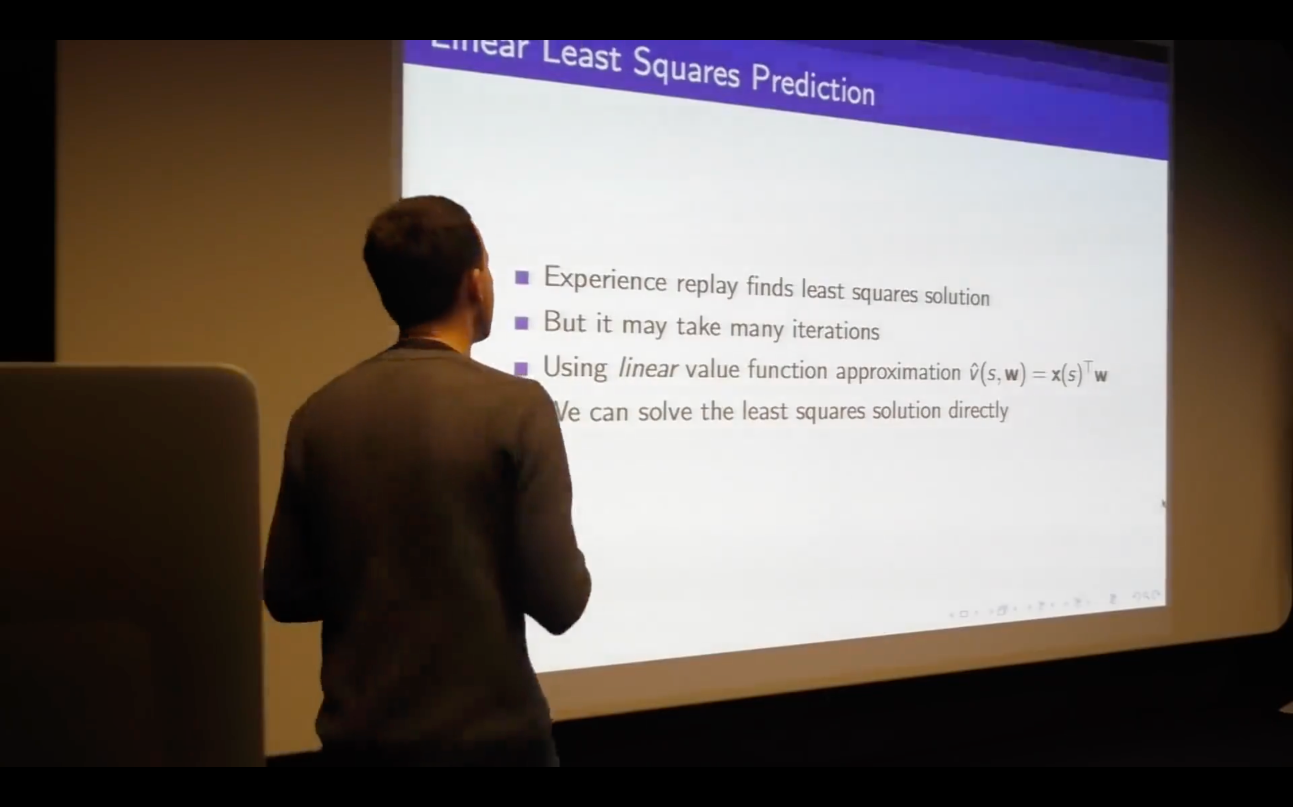
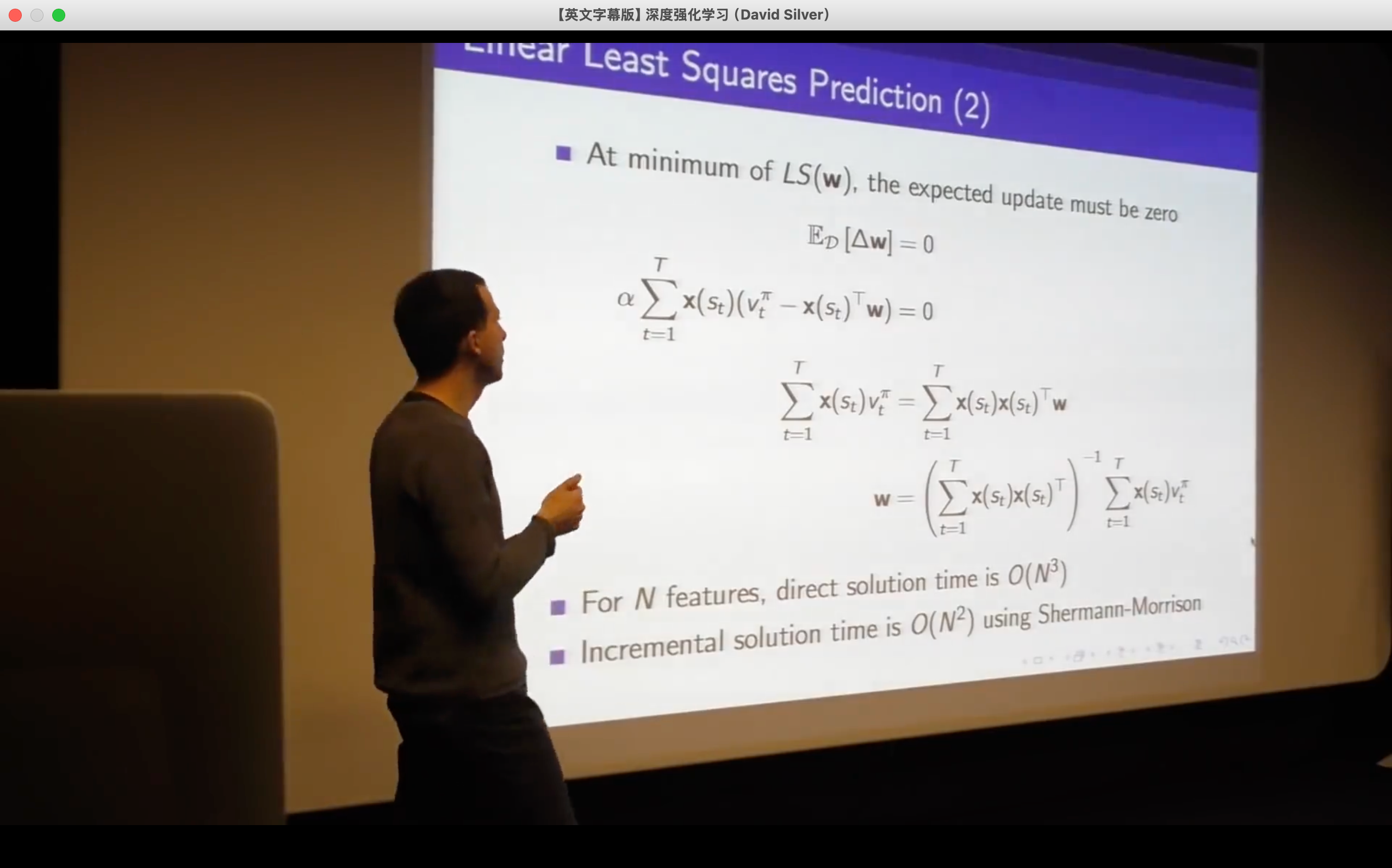
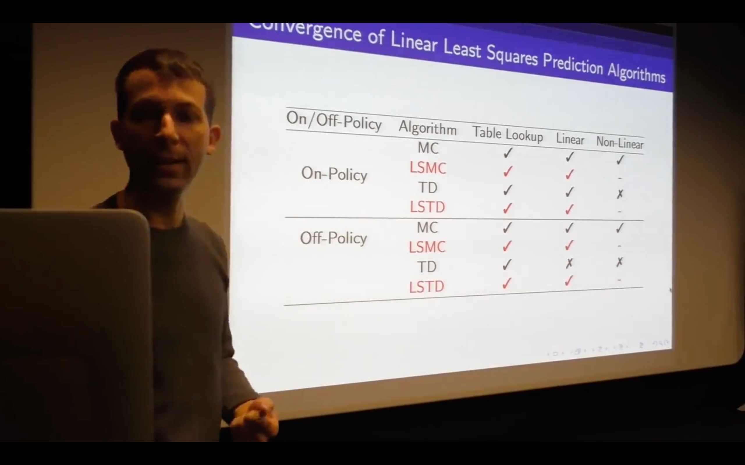
Incremental Methods
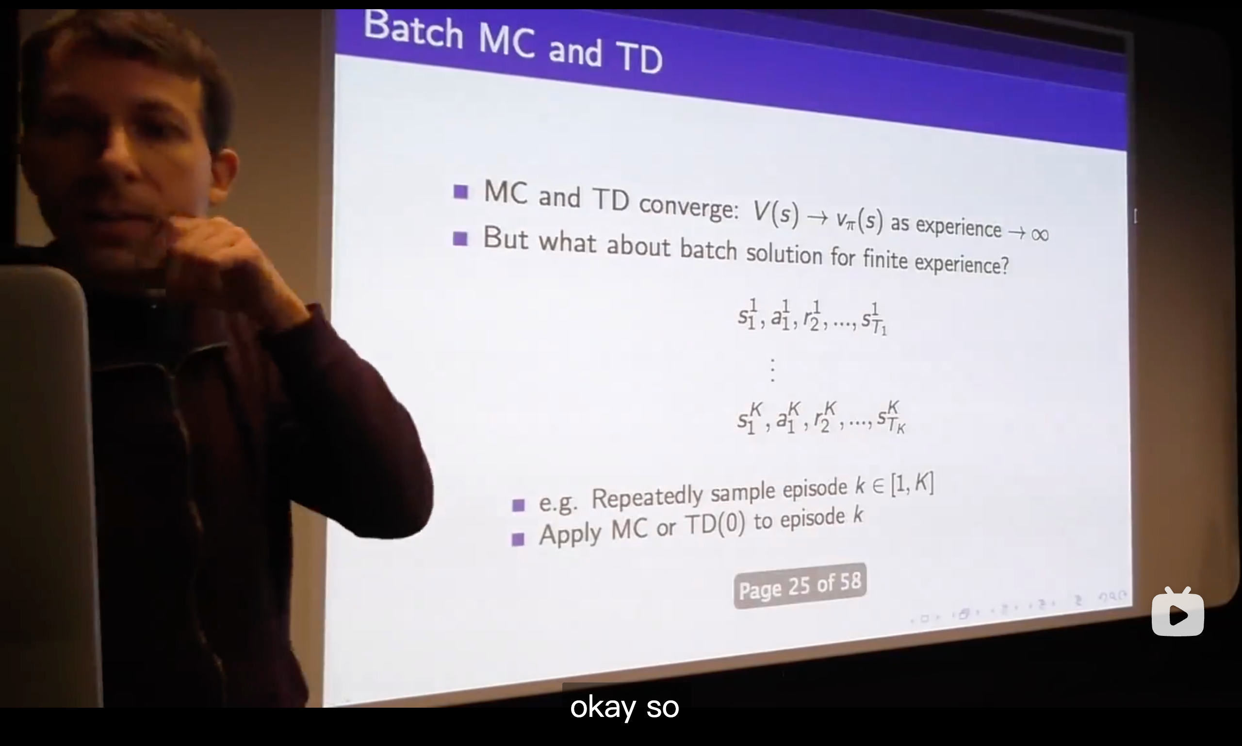
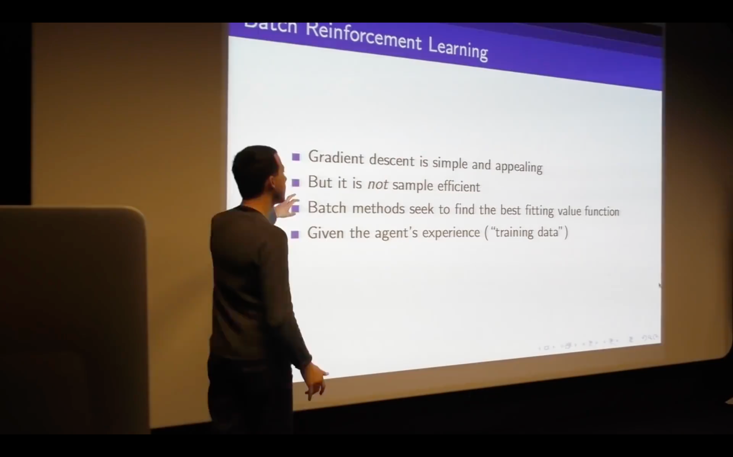
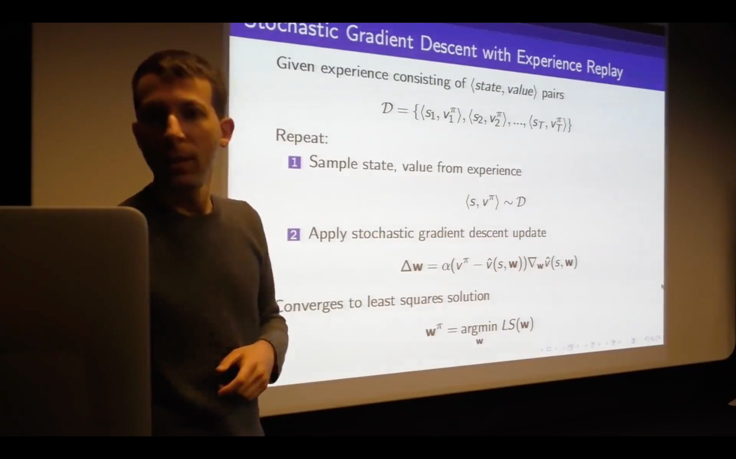
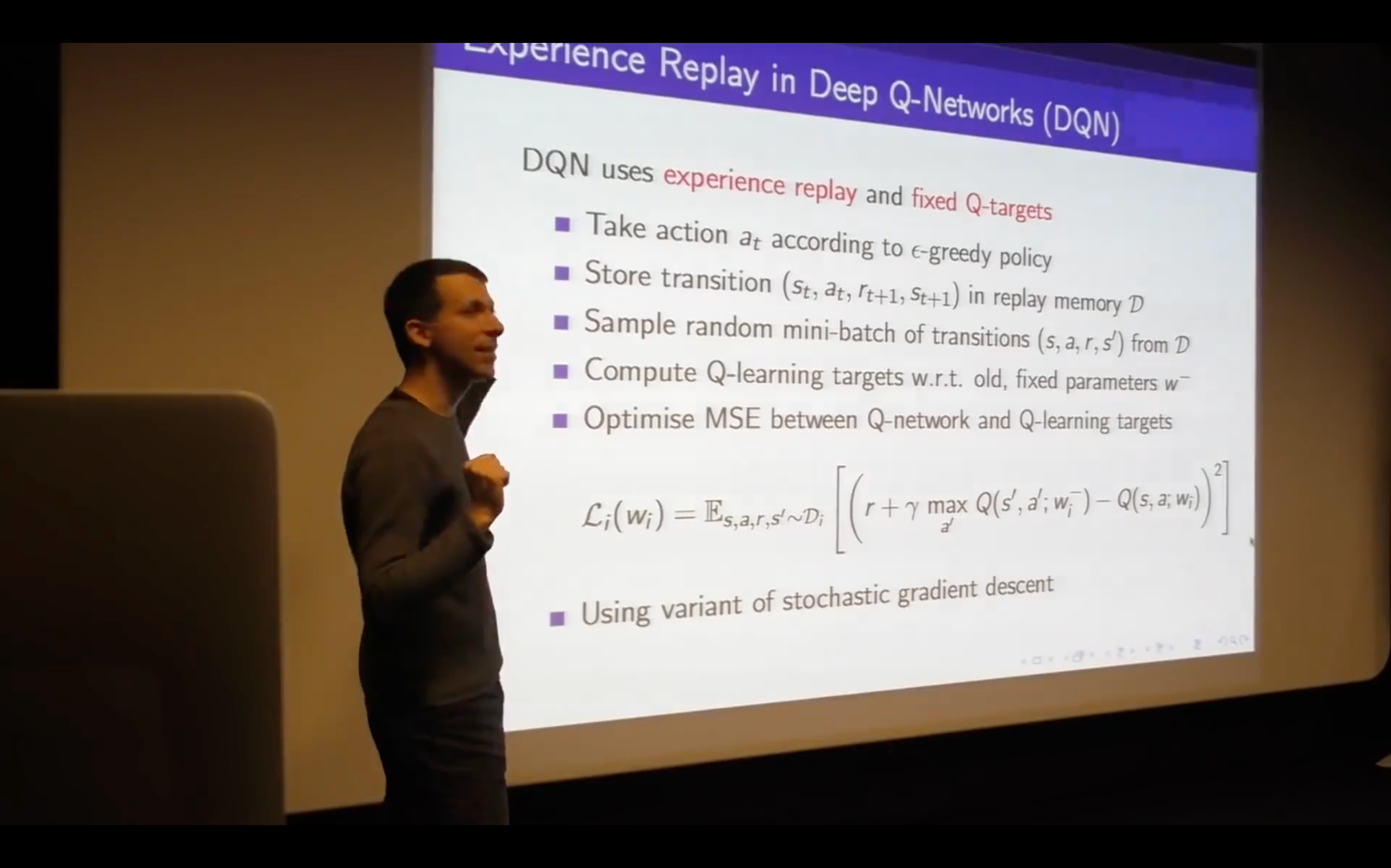
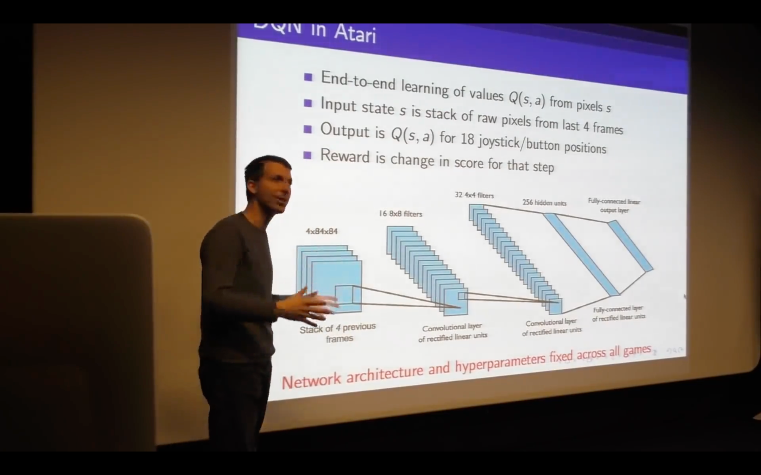
Batch Method
![]()
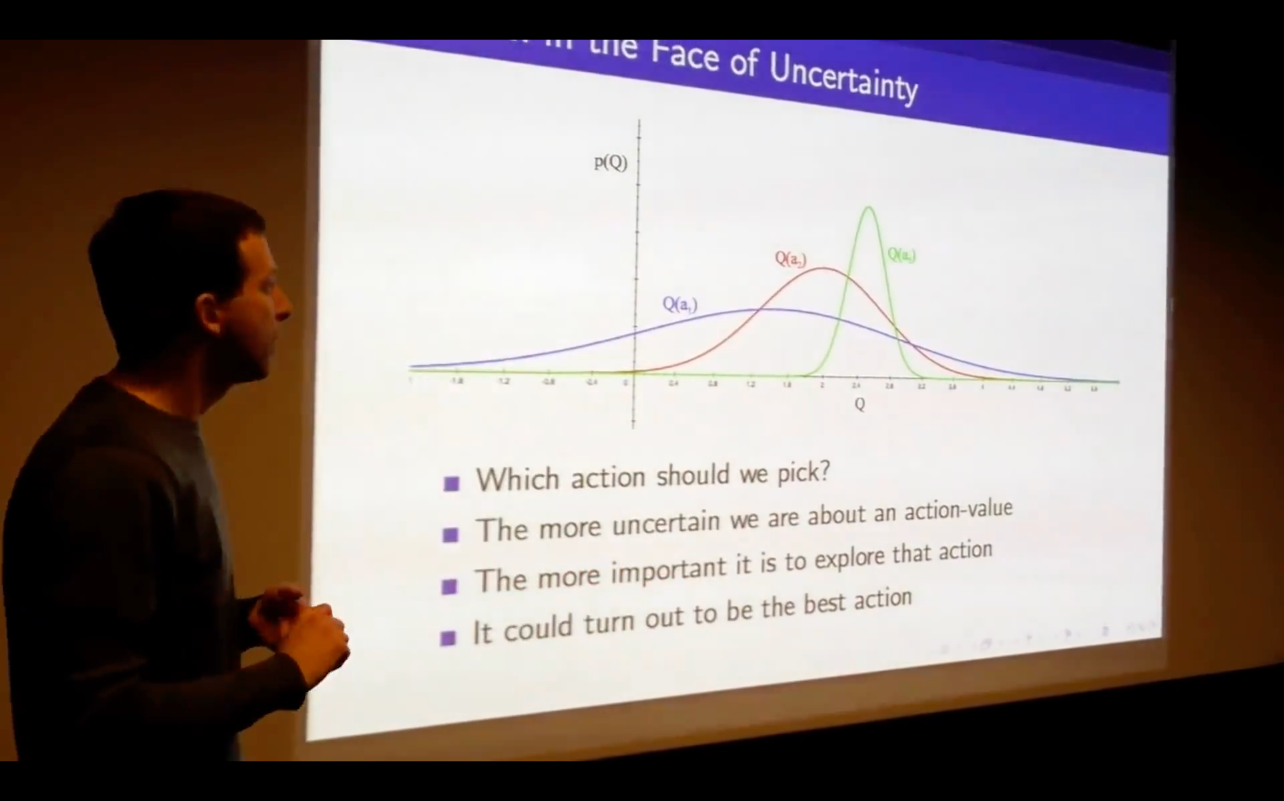
Lecture7: Exploration and Exploitation
Introduction
Three broad families:
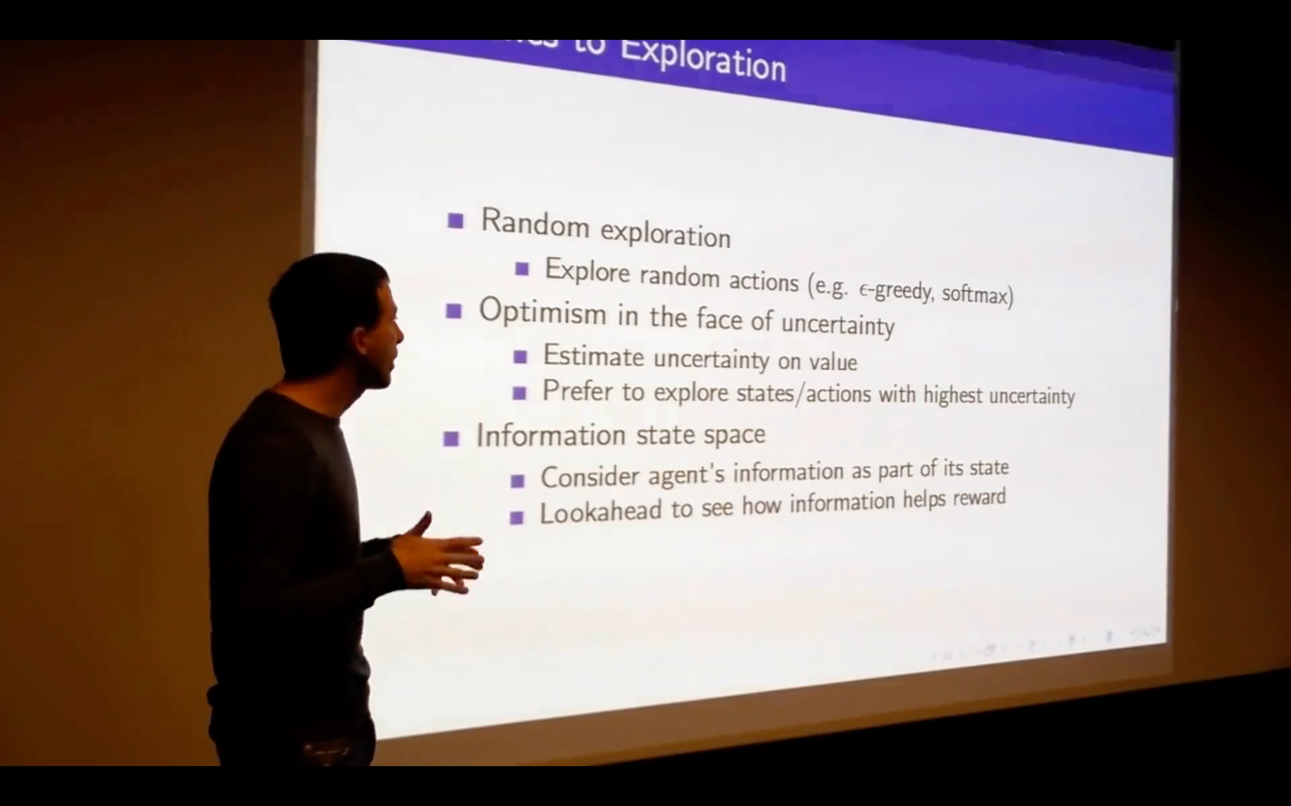
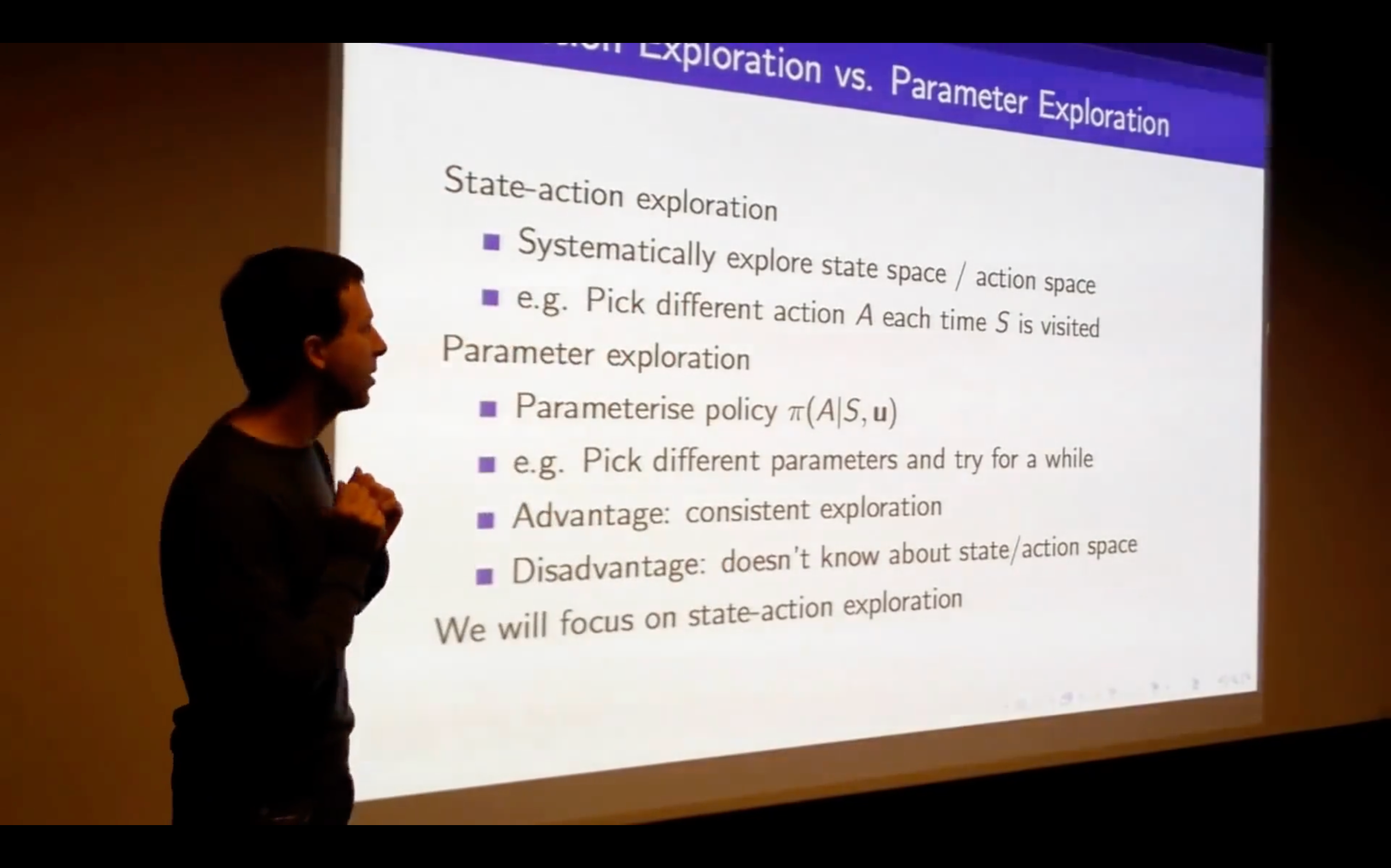
- state-action exploration / parameter exploration
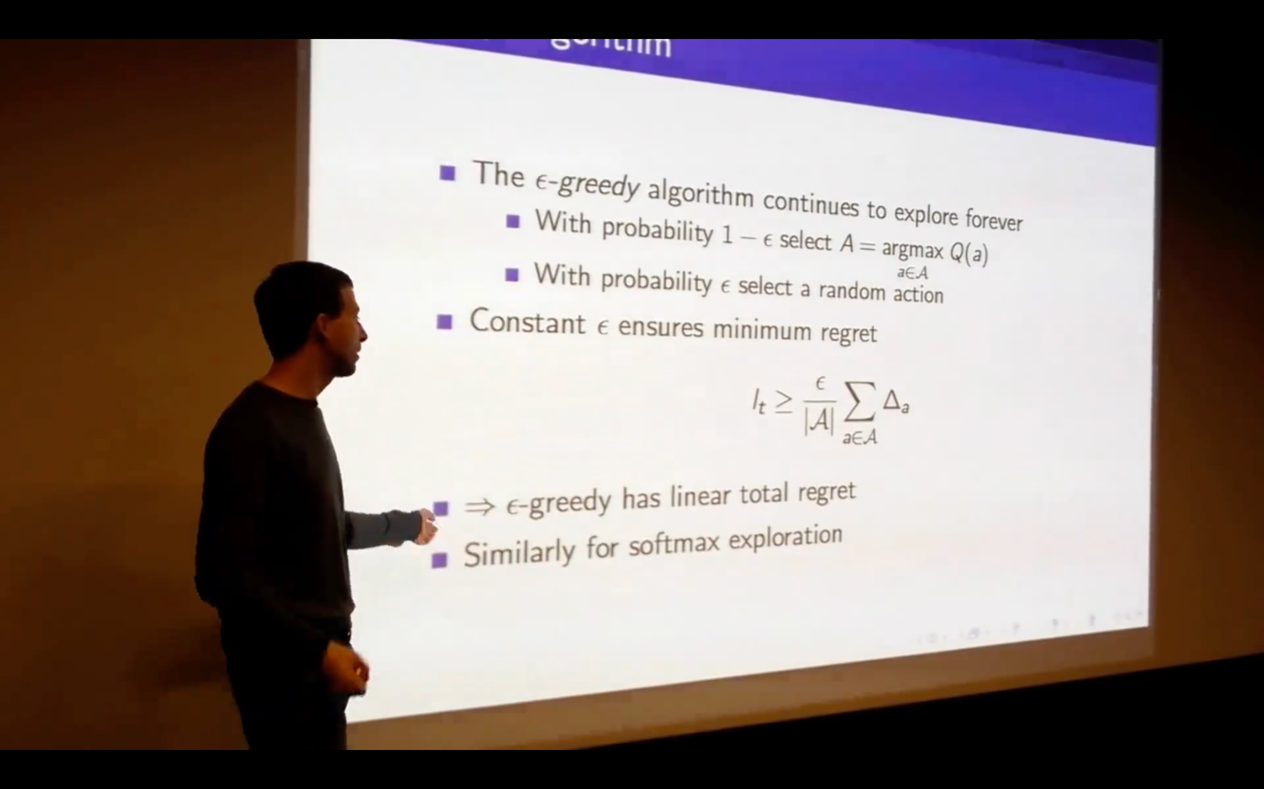
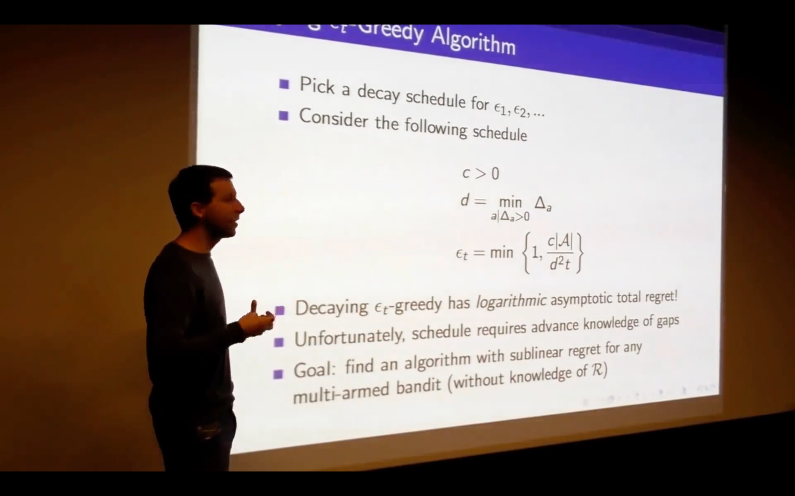
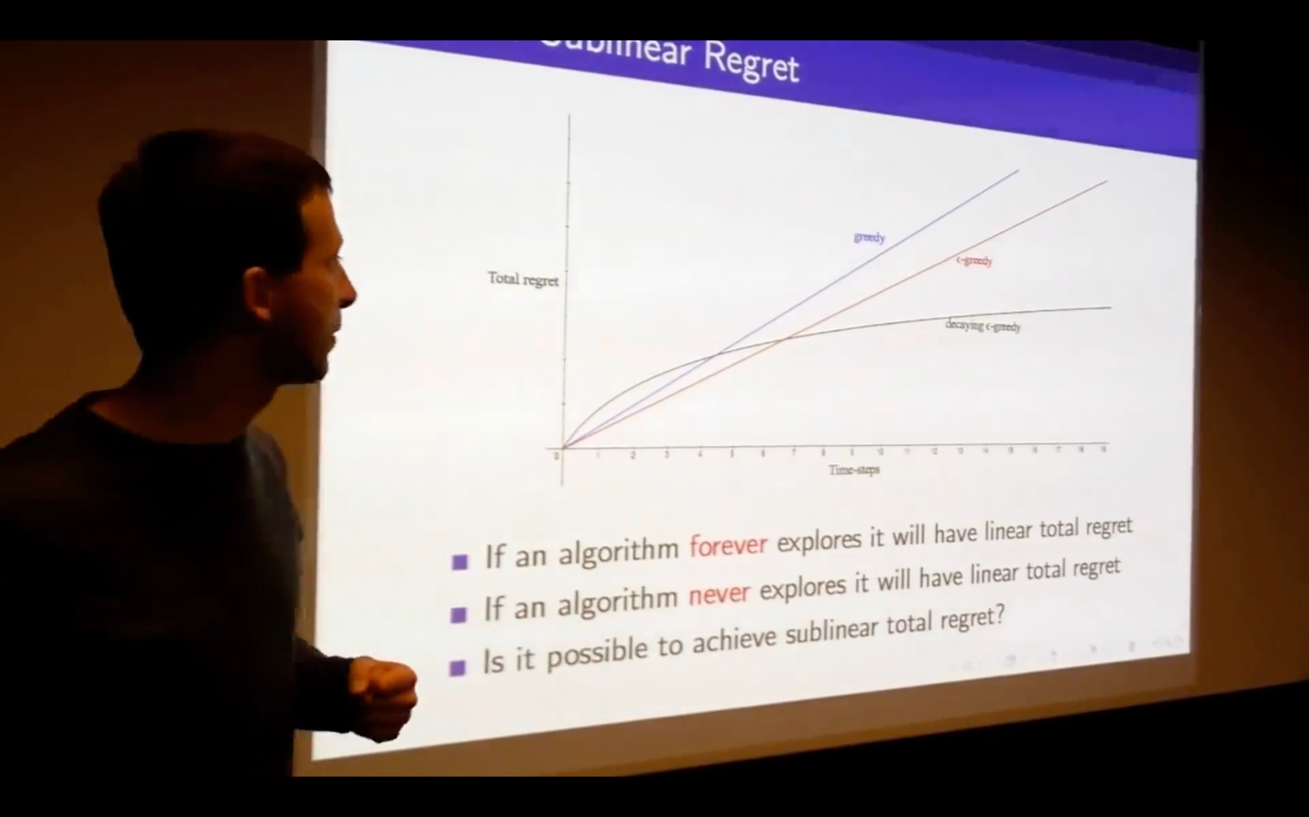
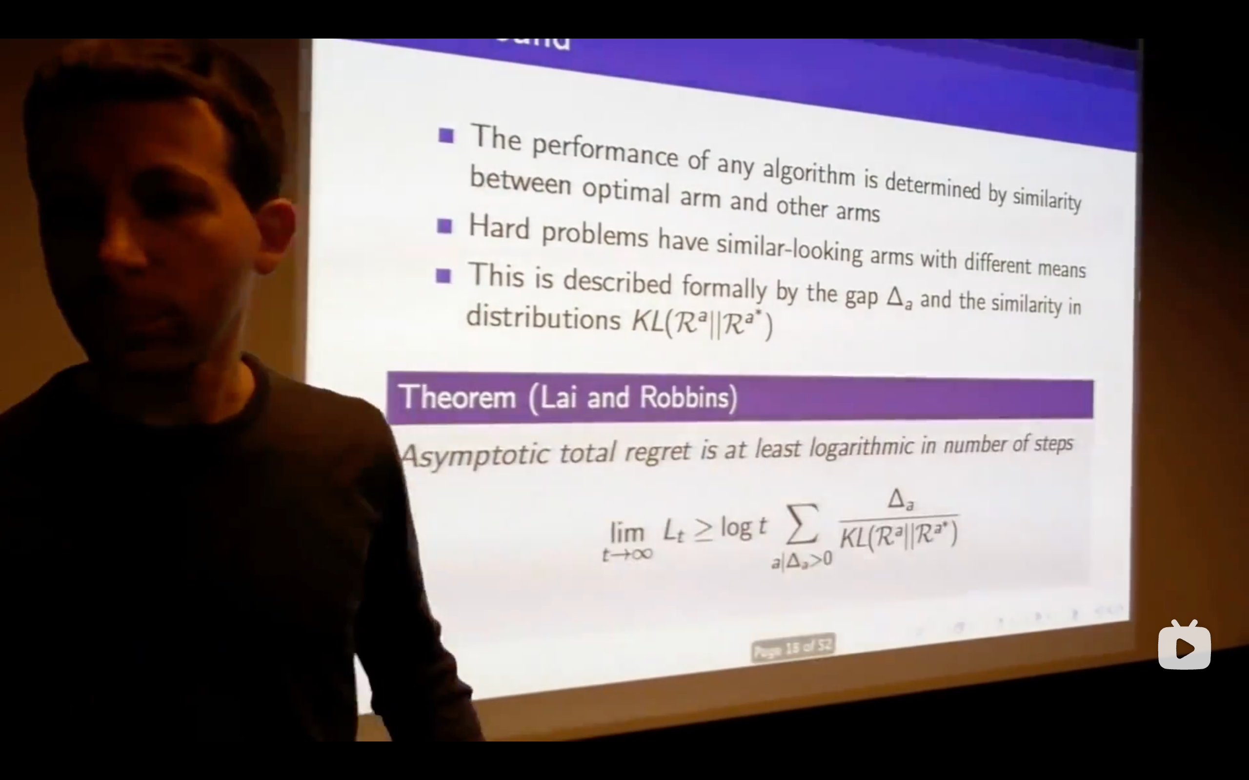
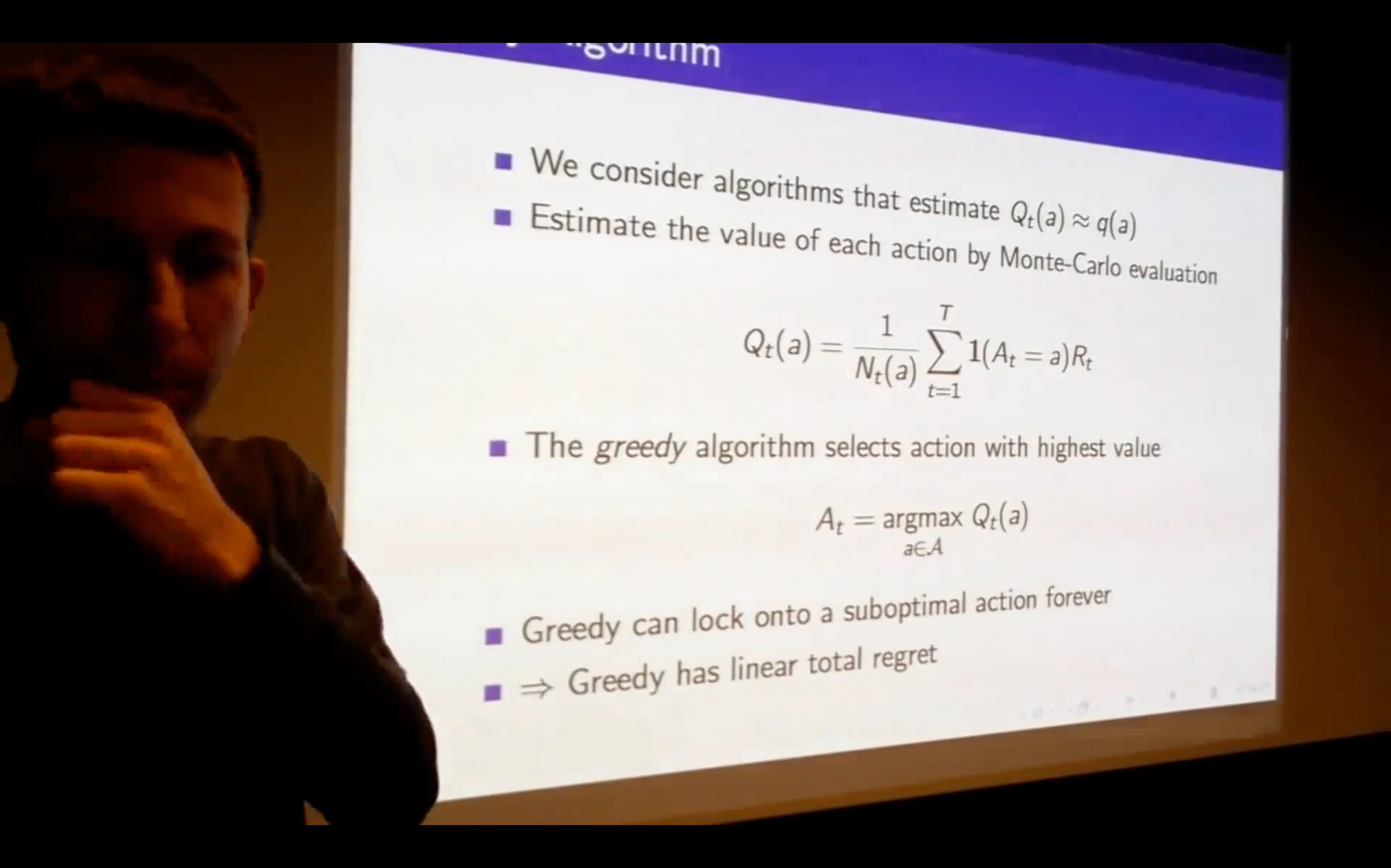
Multi-Armed Bandits
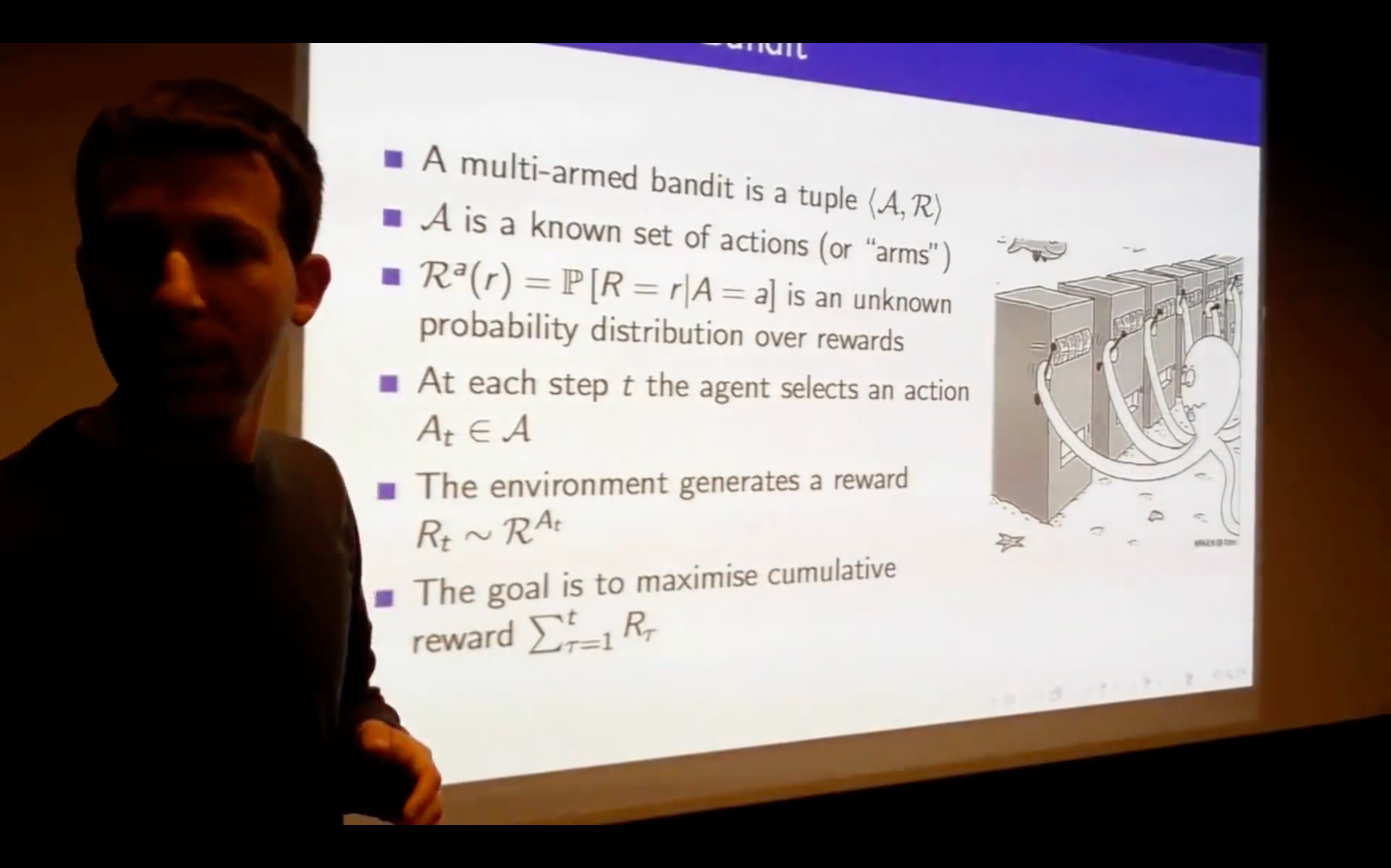
- We don't know where we start.
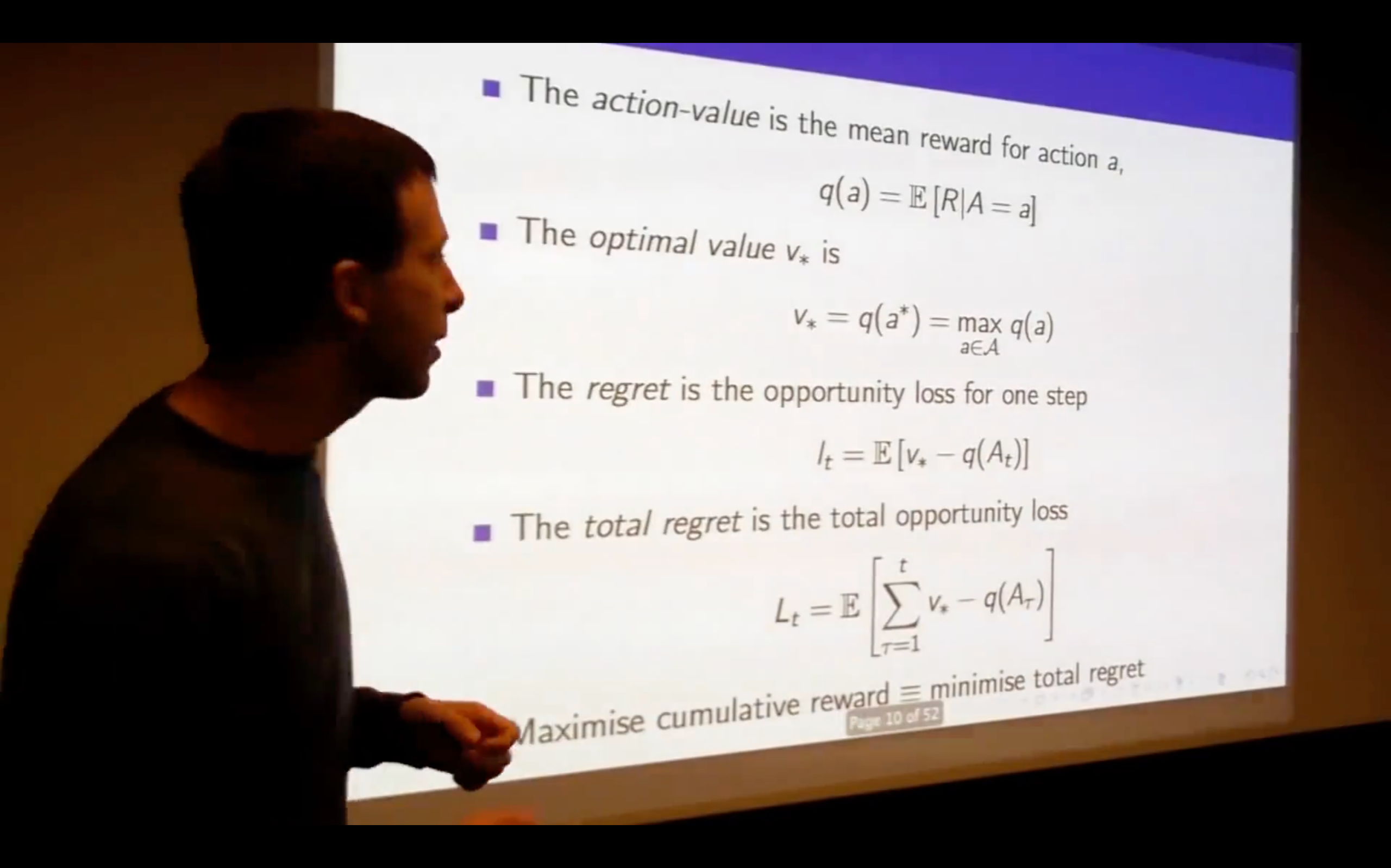
- What does the regret look like?
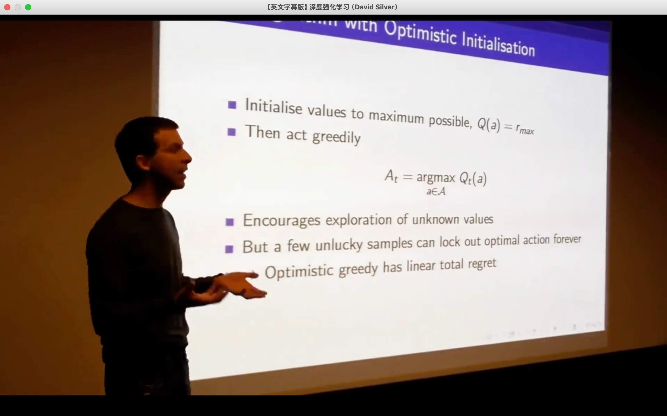
- not only initialize the value but also the count